3.3 Plots and GraphsThis section discusses various methods for generating plots of Mech output. Because Mech uses a numerical technique to solve the kinematic equations that make up a mechanism model, it is generally not possible to generate analytic expressions that represent geometric quantities in a model that are to be plotted. The best that can be done is to generate a series of discreet solutions to the mechanism model, and then use the solutions to create lists of numbers that are plotted using Mathematica's built-in data plotting routines such as ListPlot, or interpolated using Mathematica's InterpolatingFunction. 3.3.1 Example MechanismThe quick-return mechanism model that was developed in Section 3.1 is used here to demonstrate all of the plotting techniques in this chapter. The model is redefined as follows in abbreviated form.
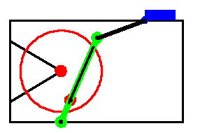
Note that a parameter crankarm has been added to the model to allow the position of the drive pin on the crank to be easily changed. Here is the entire quick-return model. A graphic of the quick-return mechanism.

3.3.2 Data PlotsTo generate a data plot, we must first generate some data. SolveMech is used to return 20 solution points as the crank is rotated through a full turn, with the crank arm length set to three units. This generates a list of 20 solutions.
Out[10]= |  |
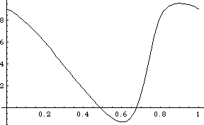
Since the primary function of the quick return mechanism is to reciprocate the slider, the X position of the slider is plotted as a function of time. Each solution rule returned by SolveMech contains a rule specifying the value of time T so a list of {x, y} pairs for ListPlot can easily be obtained with one replacement operation. Here is a plot of slider position versus time.

Out[11]= |  |
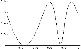
More complicated functions can also be plotted in this manner. Here is a plot of connecting rod angle versus time.

Out[12]= |  |
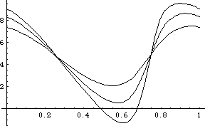
To create a series of plots while varying the value of crank arm, the Table function is used in conjunction with SolveMech to generate a nested list of solutions. Note that at each invocation of SolveMech the value of time T is taken from 0 to 1, which takes the angular coordinate of the crank  2 from 0 to 2 pi. This requires the value of 2 from 0 to 2 pi. This requires the value of  2 to jump from 2 pi back to 0 in one step at each new invocation of SolveMech, which is a rather large single step for the numerical solution method. To avoid possible numerical difficulties, the initial guesses are reset with SetGuess at each invocation of SolveMech. 2 to jump from 2 pi back to 0 in one step at each new invocation of SolveMech, which is a rather large single step for the numerical solution method. To avoid possible numerical difficulties, the initial guesses are reset with SetGuess at each invocation of SolveMech. This generates a nested list of solutions. To generate a series of plots a rather obtuse invocation of ListPlot is used. This shows a plot of slider position at varying values of crankarm.

Out[14]= |  |
3.3.3 InterpolationMathematica InterpolatingFunction objects can be used to improve the appearance of a ListPlot by smoothing out the data. Mech provides a function that facilitates the creation of InterpolatingFunction objects, by assuming a dependence on time. Mech interpolation utility. Using the quick-return mechanism model that was defined in Section 3.3.1, the plot of the connecting rod angle is reproduced using TimeInterpolate to create an InterpolatingFunction. This generates a list of solutions. This generates an InterpolatingFunction object.
Out[18]= |  |
Here is a plot of the connecting rod angle versus time.

Out[19]= |  |
|