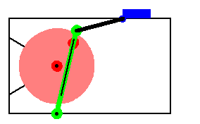
9.5 Sensitivity

MechanicalSystems' sensitivity analysis functions are used to perform linearized tolerance analysis on multibody mechanisms. Similar to the SetCouple and SolveCouple functions discussed in the previous sections, SetSensitivity and SolveSensitivity are used as a pair to build and solve SensitivitySystem objects. A planar example mechanism is developed in this section that is used to demonstrate the use of these functions.

9.5.1 Example Mechanism

The quick-return mechanism model that was developed in Section 3.1 is used here to demonstrate the use of sensitivity systems. The model is redefined as follows in abbreviated form.

Here is the entire quick-return model.

In[1]:=

Note that three parameters were added to the model that are used in the following sensitivity analysis: crankarm, which is the local x coordinate of the crankpin on the crank, drivex and drivey, which are the X and Y coordinates of the attachment point of the drive arm to the ground, respectively.

Here is a graphic of the quick-return mechanism.

9.5.2 Sensitivity to Parameter Variations

The quick-return model contains three undefined parameters: crankarm, drivex, and drivey. We wish to find the sensitivity of the location of each body in the mechanism to small changes in these parameters, about some operating point. The sensitivities are not constant, they change as the mechanism moves through a complete cycle. Thus, the maximum sensitivity at any point in a cycle is of interest.

The values of the parameters are set and the body locations are found at the initial operating point.

In[9]:=

Out[10]=

The sensitivity functions.

First, the sensitivity to variations in the crankarm parameter are found.

This builds the SensitivitySystem object.

In[11]:=

Out[11]=

This solves the SensitivitySystem object.

In[12]:=

Out[12]=

The solution returned by SolveSensitivity is identical in form to the solution returned by SolveMech[time, Solution -> Velocity]. The difference is that the velocity terms X2d, 3d, and so on, do not represent dX2/dT and d3/dT; they represent dX2/dcrankarm and d3/dcrankarm. Because the results from SolveSensitivity are returned in this form, it is possible to use any of the MechanicalSystems' output functions, differentiated once, to find the sensitivity of more complicated quantities to changes in the parameter.

Here is the sensitivity of the distance from the crank center to the slider origin to changes in crankarm.

In[13]:=

Out[13]=

Out[14]=

9.5.3 Multiple Parameters

If multiple symbols are passed to SetSensitivity, SolveSensitivity returns a nested list of solutions, one for each symbol.

Here a SensitivitySystem object is built and solved with three parameters.

In[15]:=

Here is the sensitivity of the slider location to variations in each of the parameters.

In[17]:=

Out[17]=

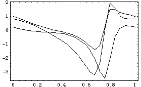
To plot the sensitivity of the slider location to changes in these three parameters, a set of solutions at several operating points is generated and used as initial conditions for SolveSensitivity.

This resets the initial guesses and seeks 25 solution points through a full turn of the crank.

In[18]:=

Now SolveSensitivity is applied with each of the position solutions serving as an initial condition.

In[20]:=

Here is a plot of the sensitivities.

In[21]:=

Out[21]=

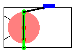
Note that the sensitivities are rather large near 3/4 turn of the crank. This is to be expected with a quick-return mechanism because of the high leverage ratio between the crank and the slider during the return stoke. The largest negative sensitivity is the sensitivity to the X coordinate of the drive arm rotational axis drivex, when the crank is at 3/4 turn.

Here is the quick-return mechanism at 3/4 turn of the crank.