|
Chapter 2
Cross-Sectional Properties of Areas
2.1 Introduction
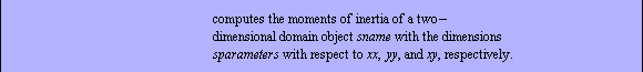
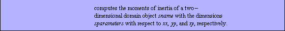
Engineering analysis and design often uses properties of plane sections in calculations. For example, in stress analysis of a beam under bending and torsional loads, you use the cross-sectional properties to determine the stress and displacement distributions in the beam cross section. In calculating the natural frequencies and mode shapes of a machine element, you also need to know the area, centroid, and various moments of inertia of a cross section. You can use the package SymCrossSectionProperties, designed to act as of an electronic handbook, to calculate properties of cross sections parametrically. Then you can use the functions in the package NumCrossSectionProperties to compute these attributes numerically.
This chapter deals with the cross-sectional properties of plane sections, both symbolically and numerically. The advantage of a symbolic output is that analytical solutions can be expressed in closed form, which enables further mathematical manipulations of the result. In the cases for which a symbolic result is not needed and/or is difficult to obtain, a numerical approach based on a triangulation scheme is used.
With the functionality of the packages SymCrossSectionProperties and NumCrossSectionProperties, you can compute various cross-sectional properties, such as area, centroid, and moment of inertia. For symbolic results, the package includes standard cross sections, such as T-sections, I-sections, and channel sections, as well as basic domain objects, such as rectangular and triangular shapes, circular and elliptical sectors, and sectors of circular and elliptical annuli. A simple procedure to combine these subdomain objects to form a complex cross section is also introduced. Using this procedure, you can easily include many practical shapes, such as L-sections, Z-sections, tampered I-sections, T-sections, and channel sections, in the calculations. The design of Structural Mechanics makes it possible to add a set of definitions for new subdomain objects to the functionality of the package. When computing the cross-sectional properties of a complex domain, numerical techniques are preferred. The numerical computations are based on a triangulation technique and an integration-in-a-triangle routine.
2.2 Symbolic Computations
2.2.1 General Remarks
The main advantage of having symbolic expressions for the cross-sectional properties of a section is that they enable the employment of powerful mathematical techniques in later stages of engineering computations. As a result of a symbolic expression, instead of finding one specific solution, you can obtain a general solution to a class of problems. With this general solution, you can evaluate a wide range of design possibilities and, consequently, reach a better design.
In Structural Mechanics, the plane sections are represented by using the function Domain.

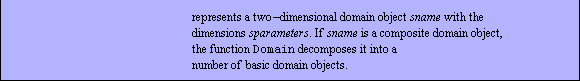
Each cross section is treated as an object or a set of objects created using the Domain function. For example, Domain[CircleSector, r, {0,  /2}] represents a data object, one-fourth of a circle with radius r, on which you can perform various operations, including SectionArea, which calculates the area of this sector. Note that angles are in radians, and the sign of an angle is described by the traditional counterclockwise direction convention. An angle described counterclockwise from the positive part of the x axis is considered positive. If it is described clockwise, the angle is considered negative. You can obtain the usage message for a domain object by typing ?objectname. For instance, ?CircleSector generates the usage message for the domain object CircleSector. /2}] represents a data object, one-fourth of a circle with radius r, on which you can perform various operations, including SectionArea, which calculates the area of this sector. Note that angles are in radians, and the sign of an angle is described by the traditional counterclockwise direction convention. An angle described counterclockwise from the positive part of the x axis is considered positive. If it is described clockwise, the angle is considered negative. You can obtain the usage message for a domain object by typing ?objectname. For instance, ?CircleSector generates the usage message for the domain object CircleSector.


The area of one-fourth of a circle with radius r is calculated by the function SectionArea, which will be described in detail shortly.
In[1]:=
In[2]:=SectionArea[Domain[CircleSector,r,{0,/2}]]
Out[2]=
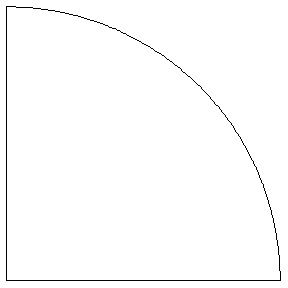
Using the Structural Mechanics' graphics primitive DomainGraphics, you can plot the shape of this sector.

In[3]:=Show[DomainGraphics[Domain[CircleSector,1,{0,/2}]]];
You can generate the same plot by using the function CrossSectionPlot.
In[4]:=

You can view the basic domains introduced in Structural Mechanics using the variable name BasicDomainList.
In[5]:=BasicDomainList
Out[5]=
The list SectionList contains built-in data objects for common cross sections generated by using domains in the list BasicDomainList.
In[6]:=SectionList
Out[6]=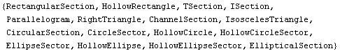
The cross sections in both lists form the collection of predefined cross sections of the package SymCrossSectionProperties. As shown in the following sections, you can easily add a new cross section to this list as either a basic domain object or a section object. When you add a new object to the package, the lists BasicDomainList and SectionList must be edited accordingly.
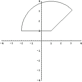
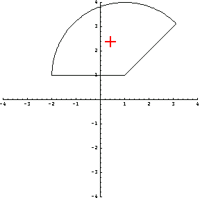
You can depict the area of a sector with the radius 1 unit, the origin at (1, 1), and the sweeping angle from /4 to .
In[7]:=
In[8]:=p1=Show[DomainGraphics[dmn],
Axes->True,
PlotRange->{{-4,4},{-4,4}}];

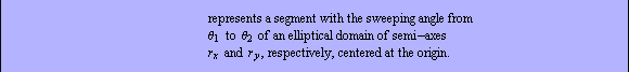


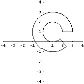
To compute the area of the following elliptical domain object, first, create a domain object for the ellipse sector. It is important to note that the arguments { , ,  } in Domain[ EllipseSector, { } in Domain[ EllipseSector, { , ,  }, { }, { , ,  } ] are the actual polar angles as opposed to the parametrization variable s in x = } ] are the actual polar angles as opposed to the parametrization variable s in x =  and y = and y = 


In[9]:=els=Domain[EllipseSector,{1,1},{3,2},{0,3/2}];
A number of option sets graphically represent this object.
In[10]:=p2=Show[DomainGraphics[els],
Axes->True,
PlotRange->{{-4,4},{-4,4}}];
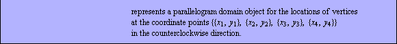
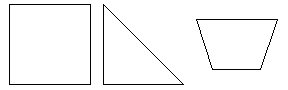
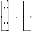
As already noted, the other three basic built-in domain objects included in Structural Mechanics are RectangularSection, RightTriangle, and Parallelogram. Here are the usage messages for the domain objects created using these section names.


As as with the ellipse sector earlier, you can generate plots of these basic domain objects.
In[11]:=tri=DomainGraphics[Domain[RectangularSection,{0,0},1,1]];
rtri=DomainGraphics[Domain[RightTriangle,{0,0},0.5,1]];
par=DomainGraphics[Domain[Parallelogram,{1,1},{4,1},{5,3},{0,3}]];
Show[GraphicsArray[{tri,rtri,par}]];
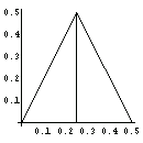
Many useful cross sections, such as hollow-rectangular, annulus, T-sections, and I-sections, can be created by arranging these basic domains as building blocks. For example, you can create the section IsoscelesTriangle domain by using two right triangles.
In[15]:=Domain[IsoscelesTriangle, b, h]
Out[15]=


In[16]:=iso=DomainGraphics[Domain[IsoscelesTriangle,{0,0},0.5,0.5]];
This shows the domain object iso.
In[17]:=Show[iso,Axes->True];
You can create the domain objects HollowCircle and HollowRectangle by removing the inner domain from the outer domain of a relevant domain object.


The domain HollowCircle is represented as the difference between two circular domains.
In[18]:=Domain[HollowCircle,{xo,yo},r1,r2]
Out[18]=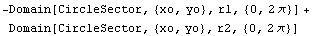
The graphical representation of composite domains with the function DomainGraphics is supported as well.
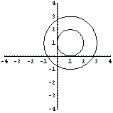
In[19]:=p3=Show[DomainGraphics[Domain[HollowCircle,{1,1},1,2]],
Axes->True,
PlotRange->{{-4,4},{-4,4}} ];
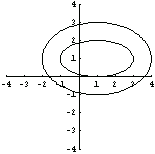
Similarly, you can use the domain HollowEllipse for elliptical hollow areas.


This graphically represents the domain HollowEllipse.
In[20]:=Show[DomainGraphics[Domain[HollowEllipse,{1,1},{2,1},{3,2}]],
Axes->True,
PlotRange->{{-4,4},{-4,4}}];
HollowRectangle is the domain name for specifying the area between two rectangular domain objects.

The rectangular hollow area HollowRectangle is represented as a composite domain object.
In[21]:=Domain[HollowRectangle,{xo,yo},b1,d1,b2,d2]
Out[21]=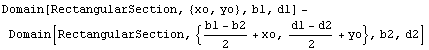
As shown here, a graphical representation for this domain object is possible.
In[22]:=Show[DomainGraphics[Domain[HollowRectangle,{0,0},2,2,3,4]]];
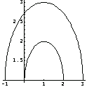
In addition to full annulus representations for circles and ellipses, a sector of an annulus is also possible. The domain name for this object is HollowCircleSector.


In[23]:=an=Domain[HollowCircleSector,{1,1},1,2,{0,7/4}]
Out[23]=
This graphically represents the sector domain an.
In[24]:=p4=Show[DomainGraphics[an],
Axes->True,
PlotRange->{{-4,4},{-4,4}}];
Similarly, the object HollowEllipseSector, a sector representation for HollowEllipse domain, is provided.


In[25]:=hes=Domain[HollowEllipseSector,{1,1},{2,1},{3,2},{0,3/2}]
Out[25]=
In[26]:=Show[DomainGraphics[hes],
PlotRange->{{-4,4},{-4,4}}];
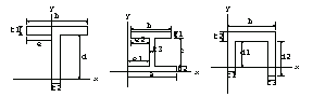
T-Section
Consider the cross sections that are commonly used in structural design. In Structural Mechanics, the T-section, I-section, and channel section are represented by built-in objects. However, as will be discussed shortly, building a new composite cross section out of the basic domain objects in BasicDomainList is a straightforward process.
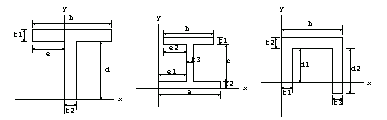
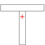
The T-section is one of the most widely used cross sections in structural design. Its domain name in Structural Mechanics is TSection.


To illustrate the dimensions of a combined section efficiently, we use the function ShowDimensions.

Here are the dimensions e,  , ,  , b, and d given in the usage message for TSection. , b, and d given in the usage message for TSection.
In[27]:=tp1=ShowDimensions[TSection];
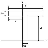
Note that by using Structural Mechanics, in addition to symmetric T-sections, you can also consider asymmetric T-sections by changing the value of the arguments. Unlike most handbooks and reference books, this feature provides you with a more flexible tool to deal with more general sections.
With this depiction of the dimensions of a T-section, you can accurately place the arguments in the domain object without any confusion.
In[28]:=tsec=Domain[TSection,2.8,0.6,1.0,6.8,3.0];
In[29]:=Show[DomainGraphics[tsec]];
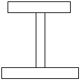
I-Section
Another type of section commonly used in engineering and design is the I-section, for which Structural Mechanics contains the built-in domain object ISection.


An I-section consists of three rectangular domain objects.
In[30]:=Domain[ISection,e1,e2,a,b,c,t1,t2,t3]
Out[30]=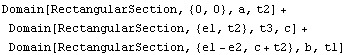
Again, the function ShowDimensions provides a graphical representation of the arguments for characteristic dimensions.
This sets the default font type and size.
In[31]:=
Out[31]=
In[32]:=tp2=ShowDimensions[ISection];
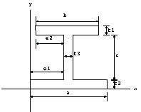
The section need not be symmetric. You can consider asymmetric I-sections by setting the variables  and and  . Here is an example with the dimensions in an appropriate length unit . Here is an example with the dimensions in an appropriate length unit  = 2.4, = 2.4,  = 2.0, a = 5.4, b = 4.4, c = 2.0, = 2.0, a = 5.4, b = 4.4, c = 2.0,  = 0.4, = 0.4,  = 0.4, and = 0.4, and  = 0.6. = 0.6.
In[33]:=isec=Domain[ISection,2.4,2.0,5.4,4.4,2.0,0.4,0.4,0.6];
In[34]:=Show[DomainGraphics[isec]];
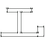
Channel Section
The channel section is also used in a wide range of applications. The object ChannelSection is reserved for general channel sections.


In[35]:=tp3=ShowDimensions[ChannelSection];
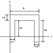
Now create a channel section with the bottom-left corner located at (1, 1) and the dimensions in an appropriate length unit b = 3,  = 1.5, = 1.5,  = 1.5, = 1.5,  = 0.5, = 0.5,  = 0.5, and = 0.5, and  = 0.5. A channel section consists of three rectangular domain objects. = 0.5. A channel section consists of three rectangular domain objects.
In[36]:=ch=Domain[ChannelSection,{1,1},3,1.5,1.5,0.5,0.5,0.5]
Out[36]=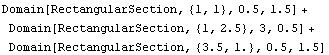
Here is how this section looks.
In[37]:=Show[DomainGraphics[ch],
Axes->True,
PlotRange->{{0,5},{0,4}},
AspectRatio->1];
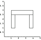
L-Section
As explained earlier, you can construct new complex cross sections by using the domain objects introduced in Structural Mechanics. You can create an L-section using two rectangular domain objects.
In[38]:=r1=Domain[RectangularSection,{0,1},1,3];
r2=Domain[RectangularSection,{0,0},4,1];
It is easy to combine these two rectangular domain objects into a composite object.
In[40]:=lsection=r1+r2;
Just like any built-in cross section, you can draw a picture of the domain object lsection.
In[41]:=Show[DomainGraphics[lsection]];
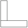
Z-Section
Now consider a Z-section consisting of three subsections.
In[42]:=r1=Domain[RectangularSection,{0,1},2,5];
r2=Domain[RectangularSection,{0,0},5,1];
r3=Domain[RectangularSection,{0,5},-3,1];
zsection=r1+r2+r3;
In[46]:=Show[DomainGraphics[zsection]];
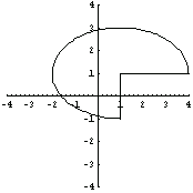
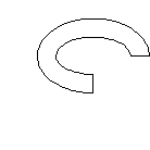
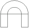
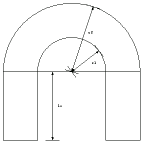
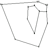
Horseshoe Cross Section
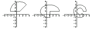
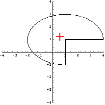
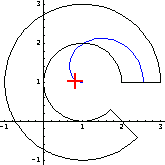
You create a horseshoe-shaped cross section using the domain objects HollowCircleSector and RectangularSection. You create the top part of the horseshoe cross section with a HollowCircleSector domain object.
In[47]:=hc=Domain[HollowCircleSector,{1,1},1,2,{0,}]
Out[47]=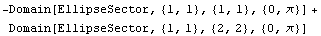
This shows the top of the cross section that you are building.
In[48]:=
Out[48]=
In[49]:=tophc=Show[DomainGraphics[hc], PlotRange ->All,Axes->True];
You use two parallel rectangular sections to build the sides of the section.
In[50]:=rec1=Domain[RectangularSection,{-1,-1},1,2];
rec2=Domain[RectangularSection,{2,-1},1,2];
In[52]:=recshc=Show[DomainGraphics[rec1+rec2],Axes->True];
As you did for the L- and Z-sections, you can create a domain object for the horseshoe cross section.
In[54]:=horseshoe=hc+rec1+rec2;
This shows the horseshoe cross section consisting of these three basic domain objects.
In[55]:=hsplot=Show[DomainGraphics[horseshoe]];
2.2.2 Area of Cross Sections
The function SectionArea in the package SymCrossSectionProperties is used to compute the area of both a built-in cross-section object and the user-defined composite domain objects. There are two ways to use this function.


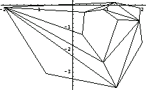
You can compute the areas of the domain objects p1, p2, and p4, which are discussed in the previous subsection, using the SectionArea function.
In[56]:=Show[GraphicsArray[{p1,p2,p4}]];
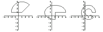
The area of the first section from the left, p1, has a radius of 1 unit length, the origin at (1, 1), and the sweeping angles from /4 to .
In[57]:=dmn=Domain[CircleSector,{1,1},3,{/4,}];
You can use consistent units in calculations. For example, the area of the sector dmn is computed as follows for the radius of 3 meters.
In[58]:=dmn=Domain[CircleSector,{1,1},3Meter,{/4,}];
In[59]:=area=SectionArea[dmn]
Out[59]=
This result is the exact value for the area of this sector. The numerical value is obtained by employing the Mathematica function N with any digit precision.
In[60]:=N[area]
Out[60]=
The area is calculated with 20-digit precision.
In[61]:=
Out[61]=
The function Convert from the Mathematica 4 Standard Add-on Packages converts the area from  to to  . This converts the area to . This converts the area to  with 10-digit precision. with 10-digit precision.
In[62]:=N[Convert[area,Inch^2],10]
Out[62]=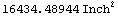
In[63]:=dmn=Domain[CircleSector,{1,1},3,{/4,}];
In[64]:=SectionArea[dmn]
Out[64]=
This is the area of the section p2.
In[65]:=els=Domain[EllipseSector,{1,1},{3,2},{0,3/2}];
In[66]:=SectionArea[els]
Out[66]=
In[67]:=N[%]
Out[67]=
Now you compute the area of the third section from the left, p3, symbolically.
In[68]:=Domain[HollowCircle,{xo,yo},R1,R2]
Out[68]=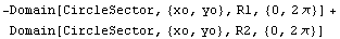
In[69]:=SectionArea[%]
Out[69]=
Equivalently, you obtain a more familiar form using Factor.
In[70]:=
Out[70]=
Next, you compute the areas of the built-in composite sections both symbolically and numerically.
In[71]:=standardsections=Show[GraphicsArray[{tp1,tp2,tp3}]];
A T-section consists of two rectangular domain objects.
In[72]:=Domain[TSection,e1,t1,t2,b,d]
Out[72]=
Here is the area of a T-section in symbolic form.
In[73]:=SectionArea[Domain[TSection,{xo,yo},e1,t1,t2,d,b]]
Out[73]=
This is the area of an I-section.
In[74]:=SectionArea[Domain[ISection,e1,e2,a,b,c,t1,t2,t3]]
Out[74]=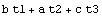
Here is the area of a channel section.
In[75]:=Domain[ChannelSection,b,d1,d2,t1,t2,t3]
Out[75]=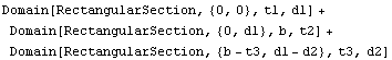
In[76]:=SectionArea[Domain[ChannelSection,b,d1,d2,t1,t2,t3 ]]
Out[76]=
The area of user-defined sections can also be calculated with SectionArea. For example, this gives the area of the horseshoe section previously created.
In[77]:=SectionArea[horseshoe]
Out[77]=
In[78]:=N[%]
Out[78]=
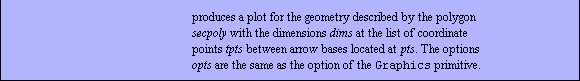
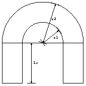
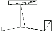
Now calculate the area in terms of the characteristic dimensions of the horseshoe. First, use the function ShowSectionDimensions to depict these dimensions.

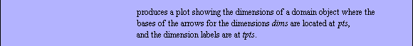

The list pts denotes the locations of the point where the arrow bases are located.
In[79]:=pts={{1,1},{1.793,1.61},{1,1},{1.630,2.901},{0.44,1},{0.44,-1.}};
The list tpts denotes the locations of the points where the parameters for dimensions, { "r1", "r2", "lx" }, are placed. Note that the orders of tpts and the dimensions must be the same for the correct correspondence.
In[80]:=tpts={{1.65,1.25},{1.55,2.15},{0.65,0.00}};
In[81]:=pp0=ShowSectionDimensions[pts,tpts,{"r1","r2","lx"} ,
DisplayFunction->Identity ];
This shows the horseshoe cross section with the specified dimensions and the aspect ratio.
In[82]:=horseshoesection=Show[pp0,hsplot,
DisplayFunction->$DisplayFunction,AspectRatio->1];
With these dimensions, you first represent the horseshoe parametrically.
In[83]:=
In[84]:=hc=Domain[HollowCircleSector,{xo,yo},r1,r2,{0,}];
In[85]:=rec1=Domain[RectangularSection,{xo-r2,yo},r2-r1,-lx];
rec2=Domain[RectangularSection,{xo+r1,yo},r2-r1,-lx];
In[87]:=horseshoe=hc+rec1+rec2
Out[87]=
Now you calculate the area of the horseshoe parametrically.
In[88]:=SectionArea[horseshoe]
Out[88]=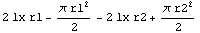
The factorization of this expression with Factor results in a compact form for the section area.
In[89]:=Factor[%]
Out[89]=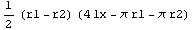
2.2.3 Centroid of Cross Sections
The centroid, or center of gravity of a plane object, is a point about which the moment of area of the object is zero, or  = 0 and = 0 and  = 0. You express the centroid of an object with the area A with the following formulas. = 0. You express the centroid of an object with the area A with the following formulas.
 and and 
Like the function SectionArea, SectionCentroid applies to both the built-in domains and user-defined composite domains.


First, compute the locations of the centroid of the previously created cross sections, p1, p2, and p4.
In[90]:=Show[GraphicsArray[{p1,p2,p4}]];
This gives the exact location of the centroid of the first section from the left, p1.
In[91]:=dmn=Domain[CircleSector,{1,1},3,{/4,}];
In[92]:=sc=SectionCentroid[dmn]
Out[92]=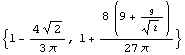
Here is the numerical value for sc with 10-digit precision.
In[93]:=N[sc,10]
Out[93]=
Next insert a plus sign using the function MarkPoint to indicate the centroid of the cross section p1.

In[94]:=Show[p1,Epilog->MarkPoint[sc]];
Here is the centroid of the second section from the left, p2.
In[95]:=els=Domain[EllipseSector,{1,1},{3,2},{0,3/2}];
In[96]:=sc=SectionCentroid[els]
Out[96]=
This is the numerical value for sc with 10-digit precision.
In[97]:=
Out[97]=
Similarly, you can easily determine and mark the centroid of the second cross section, p2.
In[98]:=Show[p2,Epilog->MarkPoint[sc]];
This is the centroid of the third section from the left, p4.
In[99]:=an=Domain[HollowCircleSector,{1,1},1,2,{0,7/4}];
In[100]:=sc=SectionCentroid[an]
Out[100]=
You can simplify this result to a shorter expression using the Mathematica function Simplify.
In[101]:=Simplify[sc]
Out[101]=
This is the numerical value for sc with 10-digit precision.
In[102]:=N[sc]
Out[102]=
As expected, when the center of this HollowCircleSector section is translated by sc, the centroid moves to the origin of the coordinate system.
In[103]:=SectionCentroid[Domain[HollowCircleSector,{1,1}-sc,1,2,{0,7/4}] ]
Out[103]=
By the definition of centroid, you would expect this result to be (0, 0). You simplify this long expression to verify that it is actually equal to {0, 0}.
In[104]:=
Out[104]=
Now compute the location of the centroid of the HollowCircleSector domain with respect to the angle determining its shape. In other words, find how the location of its centroid changes with respect to increasing the sector angle measured from the positive x axis.
You use the Mathematica ParametricPlot function to plot the results.
In[105]:=pp1=ParametricPlot[Evaluate[SectionCentroid[Domain[HollowCircleSector,{1,1},1,2,{0,ang}]]],{ang,0.001,2},PlotStyle->RGBColor[0,0,1]];
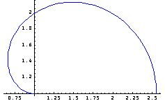
You can illustrate the location of the centroid by superimposing pp1 and the cross-section plot, p4. The plus sign in the graphic marks the centroid of the object drawn, p4.
In[106]:=Show[pp1,p4,Epilog->MarkPoint[sc],AspectRatio->1];
The centroids of built-in composite domains are computed.
In[107]:=Show[standardsections];
This is the centroid of a T-section in symbolic form.
In[108]:=Domain[TSection,{xo,yo},e1,t1,t2,b,d];
In[109]:=Clear[xo,yo,e1,t1,t2,b,d]
For the centroid of a symmetric T-section, take  to carry the x-component of the centroid to to carry the x-component of the centroid to  = =   . .
In[110]:=SectionCentroid[Domain[TSection,(b-tw)/2,t,tw,b,d]]//Together
Out[110]=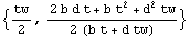
Calculate the centroid of this section for the set of numerical values previously introduced and mark the centroid on the drawing.
In[111]:=tsec=Domain[TSection,2.9,0.6,1.0,6.8,3.0];
In[112]:=SectionCentroid[tsec]
Out[112]=
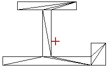
In[113]:=Show[DomainGraphics[tsec],Epilog->MarkPoint[SectionCentroid[tsec]],
PlotRange->{{-3,4},{-0,4}}];
Here you symbolically calculate the centroid of an I-section.
In[114]:=Clear[e1,e2,a,b,c,t1,t2,t3]
In[115]:=SectionCentroid[Domain[ISection,{xo,yo},e,e2,a,b,c,t1,t2,t3]]//Factor
Out[115]=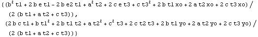
Calculate and mark the location of the centroid of the I-section.
In[116]:=isec=Domain[ISection,2.4,2.0,5.4,4.6,2.0,0.4,0.4,0.6];
In[117]:=sc=SectionCentroid[isec]
Out[117]=
In[118]:=Show[DomainGraphics[isec],Epilog->MarkPoint[sc]];
Find the centroid of a channel section.
In[119]:=Domain[ChannelSection,{xo,yo},b,d1,d2,t1,t2,t3 ]
Out[119]=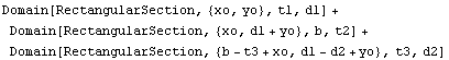
In[120]:=SectionCentroid[Domain[ChannelSection,{xo,yo},b,d1,d2,t1,t2,t3 ]]//Together
Out[120]=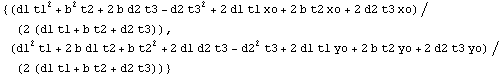
The centroid of a user-defined composite cross section is easy to compute.
In[121]:=ch1=Domain[ChannelSection,{0,0},3,1.5,1.5,0.5,0.5,0.5];
ch2=Domain[ChannelSection,{0,0},3,1.5,2.5,0.5,0.5,0.5];
In[123]:=sc1=SectionCentroid[ch1];
sc2=SectionCentroid[ch2];
As expected, the centroid is located on the positive part of the coordinate system since the right leg of the channel section is longer than the left leg.
In[125]:=Show[DomainGraphics[ch2],
Epilog->MarkPoint[sc2],
Axes->True ,
AxesOrigin->{0,0}];
SectionCentroid also calculates the centroid of user-defined sections. For example, here is the centroid of the horseshoe cross section, horseshoe, which you created previously.
In[126]:=
In[127]:=hc=Domain[HollowCircleSector,{xo,yo},r1,r2,{0,}];
In[128]:=rec1=Domain[RectangularSection,{xo-r2,yo},r2-r1,-lx];
rec2=Domain[RectangularSection,{xo+r1,yo},r2-r1,-lx];
In[130]:=horseshoe=hc+rec1+rec2
Out[130]=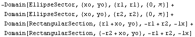
As previously noted, the domain object tophc represents the top of the cross section.
In[131]:=Show[tophc,Axes->True];
Two parallel rectangular sections are used to build the sides of the section.
In[132]:=Show[recshc,Axes->True,AspectRatio->1];
These symbols in horseshoe correspond to the dimensions, as shown here.
In[134]:=Show[pp0,hsplot,DisplayFunction->$DisplayFunction,AspectRatio->1];
From these dimensions, you can calculate the centroid of a horseshoe section parametrically.
In[135]:=SectionCentroid[horseshoe]
Out[135]=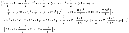
You can simplify this expression.
In[136]:=
Out[136]=
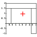
Now consider a numerical example.
In[137]:=hc=Domain[HollowCircleSector,{1,1},1,2,{0,}];
In[138]:=rec1=Domain[RectangularSection,{-1,-1},1,2];
rec2=Domain[RectangularSection,{ 2,-1},1,2];
In[140]:=horseshoe=hc+rec1+rec2;
In[141]:=sc=SectionCentroid[horseshoe]
Out[141]=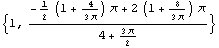
This gives the numerical value of the location of the centroid of the cross section horseshoe with 10-digit precision.
In[142]:=N[sc,10]
Out[142]=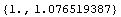
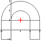
Here is the location of the centroid indicated with Mark.
In[143]:=Show[hsplot,Epilog->MarkPoint[sc],Axes->True];
2.2.4 Moments of Inertia
In this section, you can obtain the expressions for the moments of inertia, products of inertia, and polar moments of inertia of various cross-sectional domains using the functions provided in Structural Mechanics. Functions for calculating these moments of translated and rotated domains are also included. By using the function SectionArea along with the functions introduced in this section, you can compute the radius of gyration of a section.
Here is a list of the functions available in Structural Mechanics for calculating moments of inertia and other related quantities.
In[144]:=?Section*Moment*
SectionInertialMoments SectionPolarInertialMoments
SectionMomentsRotate SectionPolarMomentsRotate
SectionMomentsTranslate SectionPolarMomentsTranslate
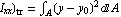
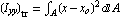
The moments of inertia with respect to the x and y axes for a planar geometry with the area A are defined as follows.
 and and 
Similarly, the cross product of inertia of an area is given as follows.

The definition of the polar moment of inertia of an area is given below.
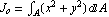 = = = =  + + 


You compute the moments and the products of inertia of a rectangular section about an axis system originating at the lower-left corner of the rectangle.
In[145]:=SectionInertialMoments[Domain[RectangularSection,{0,0},b,d]]
Out[145]=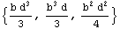
Using the following, you can generate a set of replacement rules for future use.
In[146]:=
Out[146]=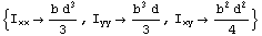
The centroid of this section is at the point (b/2, d/2).
In[147]:=SectionCentroid[Domain[RectangularSection,{0,0},b,d]]
Out[147]=
In order to calculate the section moments and product moment about the coordinate system translated to the section centroid, you need to slide the centroid point in the opposite direction by the coordinates of the centroid, that is, (-b/2, -d/2).
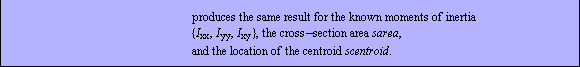
In[148]:=smi=SectionInertialMoments[Domain[RectangularSection,{-b/2,-d/2},b,d]]
Out[148]=
The replacement rules for the moments of inertia are formed.
In[149]:=
Out[149]=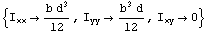
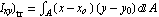
The functions for calculating the moments of inertia of a shifted cross section are available. The moments of inertia of a cross section in an axes system translated by  , ,  ) are computed by evaluating the following integrals over area A. ) are computed by evaluating the following integrals over area A.
( , ,  and and
(


In[150]:=SectionMomentsTranslate[Domain[RectangularSection,b,d],{b/2,d/2}]
Out[150]=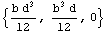
Here are the radii of gyration with respect to this axis system.
 and and 
This calculates the radii of gyration for a rectangular section.
In[151]:=Sqrt[smi/SectionArea[RectangularSection,b,d]]
Out[151]=
Equivalently, find the numerical values of the coefficients with 10-digit precision.
In[152]:=N[%,10]
Out[152]=
Since symbols b and d are dimensions and thus they are positive real numbers, you can further simplify this expression.
In[153]:=PowerExpand[%]
Out[153]=
It can be easily proven that the section moments of inertia ( and and  )are minimum about the coordinate system whose origin is at the centroid of the section. To verify this for a rectangular cross section, translate the coordinate system by ( )are minimum about the coordinate system whose origin is at the centroid of the section. To verify this for a rectangular cross section, translate the coordinate system by ( , ,  )and calculate the inertias. )and calculate the inertias.
In[154]:=
Out[154]=
This result shows that the origin of the coordinate system is the centroid of the section since the moments of inertia are minimum for  = 0 and = 0 and  = 0. = 0.
T-Section
Calculate and simplify the centroid of a T-section for a set of parametric dimensions.
In[155]:=sc=SectionCentroid[Domain[TSection,{0,0},(b-tw)/2,t,tw,b,d]]//Simplify
Out[155]=
As expected, the location of the cross section is shifted by sc. Note that -sc indicates that the cross section, not the coordinate system, is shifted.
In[156]:=SectionCentroid[Domain[TSection,-sc,(b-tw)/2,t,tw,b,d]]//Together
Out[156]=
Here are the moments and cross product of inertia about the coordinate system whose origin is located at the section centroid.
In[157]:=SectionInertialMoments[TSection,-sc,(b-tw)/2,t,tw,b,d]//Together
Out[157]=
You obtain the same result by translating the coordinate system by sc. Instead of shifting the cross section with respect to the coordinate system, the function SectionMomentsTranslate shifts the coordinate system.
In[158]:=SectionMomentsTranslate[Domain[TSection,(b-tw)/2,t,tw,b,d],sc]//Together
Out[158]=
In[159]:=
Out[159]//TableForm=
Next you can calculate the moments of inertia of a rotated section.


In[160]:=mi=SectionInertialMoments[Domain[RectangularSection,{x1,y1},b,d]]//Together
Out[160]=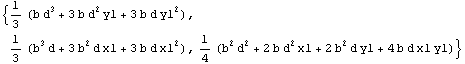
In[161]:=smr=SectionMomentsRotate[Domain[RectangularSection,{x1,y1},b,d], ]//Together ]//Together
Out[161]=


In[162]:=SectionPolarInertialMoments[Domain[TSection,-sc,(b-tw)/2,t,tw,b,d]]//Together
Out[162]=
By definition, the polar moments of inertia are the sum of  and and  . Thus, the difference between this result and . Thus, the difference between this result and  must vanish. must vanish.
In[163]:=
Out[163]=
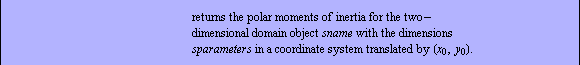
Similarly, the function SectionPolarMomentsTranslate computes the polar section moments of inertia.


2.2.5 Principal Axes
For a cross section, there exists a coordinate system  in which the product moment of inertia vanishes, that is, in which the product moment of inertia vanishes, that is,  = 0. You can determine this coordinate system by either rotating the original coordinate system = 0. You can determine this coordinate system by either rotating the original coordinate system  , with its origin located at the centroid of the cross section, or rotating the cross section with respect to the same original coordinate system (Oxy). In Structural Mechanics, the latter is adopted in the function DomainPrincipalAxesDirections, while the former can also easily be performed. , with its origin located at the centroid of the cross section, or rotating the cross section with respect to the same original coordinate system (Oxy). In Structural Mechanics, the latter is adopted in the function DomainPrincipalAxesDirections, while the former can also easily be performed.


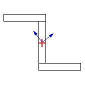
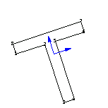
Now define a Z-section and illustrate its principal axes.
In[164]:=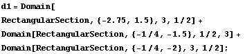
In[165]:=
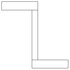
The origin of the geometry is at the centroid of the section due to the symmetry.
In[166]:=
Out[166]=
This calculates the two vectors defining the orientation of the principal axes.
In[167]:=
Out[167]=


Using the function MarkAxisSystem, you can show these directions. The axis system is shown in blue by prepending the color graphics directive RGBColor[0,0,1] to the object created by MarkAxisSystem.
In[168]:=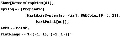
Rotate the section by the orientations of the principal axes and calculate the moments of inertia. Note that the rotation angles are negated since it is the section that is rotated, not the coordinate systems.
In[169]:=
Out[169]=
In[170]:=
Out[170]=
2.3 Numerical Computations
2.3.1 General Remarks
While you can add a set of new subdomains in order to enhance the symbolic functionality of Structural Mechanics, a numerical result may be sufficient for a quick calculation of geometric attributes of a complex shape. Include for this purpose are a numerical scheme based on a triangulation method and an integration-in-a-triangle routine. The functionality of Structural Mechanics is not limited to convex domains; therefore, you can also consider the domains that contain openings (e.g., holes) by using the tools presented here.
This subsection considers a simple domain that is used as an example to introduce some ideas behind the package NumCrossSectionProperties, a T-section, an unconventional I-section, a complex section, and a section with an opening. After these geometries are introduced, the areas, centroids, moments of area, and cross-product moments are calculated.
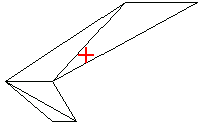
Example 1: A Simple Domain
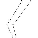
First, consider the very simple domain formed by the following coordinate points.
In[171]:=ptsSimple={{0, 0},{1,-2},{1.5,-2},{1,0},{4,4},{2.5,4}}
Out[171]=
The function PolygonPlot depicts this domain with its numbered vertices.

In[172]:=ppSimple=PolygonPlot[ptsSimple];
You use the function PolygonArea to determine the area of a polygon from its triangulation.

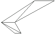
You compute the area of the polygon defined by the coordinate points ptsSimple after the interior of the polygon is triangulated using the function TriangleCoordinates.

This triangulates the polygon. Each three-element list is the coordinates of a triangle.
In[173]:=
Out[173]=
You use PolygonArea to calculate the area of the polygon from its triangulated coordinates.
In[174]:=PolygonArea[%]
Out[174]=
Next you partition this domain into triangles using the function PolygonTriangulate.

In[175]:=ptsSimple
Out[175]=
In[176]:=ptSimple=PolygonTriangulate[ptsSimple]
Out[176]=
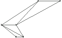
This output indicates that the vertices 1, 2, and 3 form a triangle, and so on. The function TriangulationPlot produces a plot showing the triangulation.


Now draw the graph of the triangulation of this polygon.
In[177]:=tpSimple=TriangulationPlot[ptsSimple ];
Unlike PolygonPlot, TriangulationPlot does not number the nodal points. However, the superimposition of two plots produces the nodal number on the triangulated polygon.
In[178]:=Show[tpSimple,ppSimple];
The winding number for a polygon and a point are calculated to determine if the point is inside the polygon. You use the function WindingNumber for this purpose.

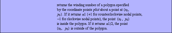
This tells you that the point ( ) is located inside the area specified by the polygon ptsSimple. ) is located inside the area specified by the polygon ptsSimple.
In[179]:=
Out[179]=
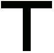
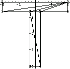
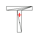
Example 2: A T-Section
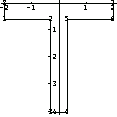
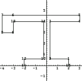
The following list, ptsTsection, represents the coordinates of a polygon forming a typical T-section.
In[180]:=ptsTsection={{-2,-0.6},{-0.3,-0.6},{-0.3,-4},{0.3,-4},
{0.3,-0.6},{2,-0.6},{2, 0},{-2, 0}};
This T-section may be visualized in many different ways. First, you use the Mathematica built-in graphic primitives.
In[181]:=Show[Graphics[Polygon[ptsTsection]],AspectRatio->1];
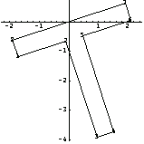
PolygonPlot generates a graph with numbered nodal points.
In[182]:=ppTsection=PolygonPlot[ptsTsection,Axes->True];
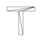
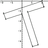
The function PolygonTriangulate calculates a triangulation of the cross section given by the polygon ptsTsection.
In[183]:=PolygonTriangulate[ptsTsection]
Out[183]=
This is how a particular triangulation looks.
In[184]:=tpTsection=TriangulationPlot[ptsTsection,
PlotRange->{{-3,3},{-5,1}},
AspectRatio->1];
Superimposing ppTsection and tpTsection adds the node number to the triangulated cross section.
In[185]:=Show[ppTsection, tpTsection];
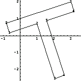
To rotate a group of points with respect to the reference point by a specified angle, you can use the function PolygonRotate.


This is a rotation of the section about the origin of the coordinate system (0, 0) by /10.
In[186]:=PolygonPlot[PolygonRotate[ptsTsection,{0,0},N[/10]],Axes->True];
Now rotate it about the point (2, 0).
In[187]:=PolygonPlot[PolygonRotate[ptsTsection,{2,0},N[/10]],Axes->True];
PolygonTranslate is employed to translate a cross section.


This translates the previously rotated polygon by (1, 2).
In[188]:=
Example 3: An Unconventional I-Section
By taking advantage of the triangulation function, you can deal with complex and irregular cross-section geometries. In this example, consider an I-section with an additional attachment.
In[189]:=ptsIsection={{-2,-0.6},{-0.3,-0.6},{-0.3,-4},
{-3,-4},{-3,-4.6},{3,-4.6},{4,-4.6},{4,-3},
{3,-3},{3,-4},{0.3,-4},{0.3,-0.6},{2,-0.6},{2,0},{-2,0}};
In[190]:=ppIsection=PolygonPlot[ptsIsection];
Here is the depiction of this triangulation of ptsIsection.
In[191]:=tpIsection=TriangulationPlot[ptsIsection];
You rotate this I-section with respect to the origin (0, 0) by 180 degrees and generate the new coordinates of the nodal points.
In[192]:=rotatedI=PolygonRotate[ptsIsection,{0,0},N[]]//Chop
Out[192]=
This is the rotated section.
In[193]:=PolygonPlot[rotatedI,Axes->True];
Example 4: A Complex Domain with an Opening
As noted earlier, the triangulation function in Structural Mechanics can handle domains with openings. Now consider a complex shape with an opening.
In[194]:=ptsComplex={{-0.770, -3.06}, {1.25, -3.69}, {1.99, -1.7},
{1.91, -0.70}, {1.3, -0.67}, {0.88, -2.57},
{0.28, -1.33}, {0.34, -0.31}, {0.88, -0.19},
{1.3, -0.67}, {1.91, -0.70}, {1.93, -0.12},
{1.2, 0.13}, {-1.96, -0.09}};
This shows the domain.
In[195]:=Show[Graphics[Polygon[ptsComplex]]];

As the following graph shows, you create the opening in this cross section by including overlapping sides to form the polygon. In this example, the points 4 and 11 and the points 5 and 10 are of the same coordinates. Note that the plot generated by the function PolygonPlot shows only the points 4 and 5.
In[196]:=p2=PolygonPlot[ptsComplex];
Here you can generate and plot the triangulation of the region with the opening.
In[197]:=tpComplex=TriangulationPlot[ptsComplex,Axes->True];
Use the function WindingNumber to verify that the opening is considered to be outside of the area specified by the polygon. The point (1, -1) is inside the opening.
In[198]:=
Out[198]=
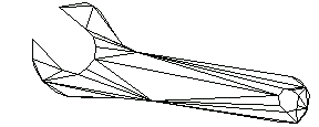
Example 5: A Practical Application—A Wrench
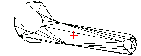
Now consider a practical plane shape: a wrench. Here is the list of coordinate points forming a wrench.
In[199]:=ptsWrench={
{0.845,0.224},{0.385,0.290},{0.344,0.307},{0.324,0.332},{0.272,0.399},{0.253,0.413},{0.229,0.421},{0.152,0.411},{0.232,0.352},{0.253,0.330},{0.261,0.303},{0.256,0.273},{0.232,0.246},{0.207,0.232},{0.162,0.243},{0.072,0.325},{0.072,0.273},{0.078,0.248},{0.102,0.214},{0.140,0.185},{0.177,0.171},{0.253,0.170},{0.327,0.170},{0.427,0.162},{0.812,0.104},{0.859,0.102},{0.881,0.121},{0.890,0.140},{0.860,0.150},{0.856,0.137},{0.826,0.132},{0.807,0.149},{0.805,0.174},{0.821,0.192},{0.845,0.190},{0.862,0.176},{0.860,0.150},{0.890,0.140},{0.896,0.179},{0.887,0.195},{0.868,0.215}};
Many sampling points are needed to represent the smooth edges.
In[200]:=Show[Graphics[Polygon[ptsWrench]], AspectRatio->.4, Axes->True];
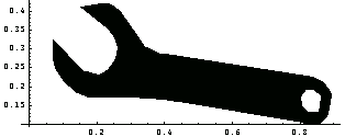
Here is the polygon showing the nodal points and their numbers.
In[201]:=ppWrench=PolygonPlot[ptsWrench];
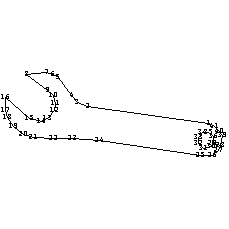
Although the number of points in the polygon is quite high, you can easily generate a triangulation.
In[202]:=tpWrench=TriangulationPlot[ptsWrench,AspectRatio->.4];
2.3.2 Areas of Cross Sections
Use the function PolygonArea to compute the area covered by a polygon. PolygonArea is based on the triangulation scheme.

Now compute the areas of the regions discussed earlier. Note that the argument of the function AreaPolygon is a triangulation with coordinates. This argument is a list of lists containing coordinates of three vertices that form a triangle. The actual coordinates, instead of the vertex numbers, are the elements of the argument. The function TriangleCoordinates produces this output from the points by calling the triangulation function. The main advantage of this approach is to eliminate unnecessary triangulation for the same polygon for different purposes, such as calculating area and centroid.
Here is the area of the simple domain.
In[203]:=tcSimple=TriangleCoordinates[ptsSimple];
In[204]:=PolygonArea[tcSimple]
Out[204]=
Here is the area of the T-section.
In[205]:=tcTsection=TriangleCoordinates[ptsTsection];
In[206]:=PolygonArea[tcTsection]
Out[206]=
This is the area of the unconventional I-section.
In[207]:=tcIsection=TriangleCoordinates[ptsIsection];
In[208]:=PolygonArea[tcIsection]
Out[208]=
Next compute the area of the complex domain with an opening.
In[209]:=tcComplex=TriangleCoordinates[ptsComplex];
In[210]:=PolygonArea[tcComplex]
Out[210]=
Here is the area of the wrench profile.
In[211]:=tcWrench=TriangleCoordinates[ptsWrench];
In[212]:=PolygonArea[tcWrench]
Out[212]=
2.3.3 Centroids of Cross Sections
In this section, you compute the coordinates of the centroid locations of the cross sections introduced in Section 2.3.1, and mark them on the triangulation graphs. You find the location of the center of gravity of an area described by a polygon by using the function PolygonCentroid.

In[213]:=pc=PolygonCentroid[tcSimple]
Out[213]=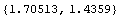
Using the function Mark, you can mark the location of the centroid as you did for the domain names.
In[214]:=Show[tpSimple, Epilog->MarkPoint[pc]];
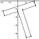
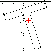
After you compute the location of the centroid of the previously introduced T-section , it is marked on the triangulation of the shape.
In[215]:=pc=PolygonCentroid[tcTsection]
Out[215]=
In[216]:=Show[tpTsection,Epilog->MarkPoint[pc],PlotRange->{{-3,3},{-5,1}},AspectRatio->1];
As mentioned earlier, you can rotate a section by an angle about a point on the plane. The list rotptsTsection contains the coordinates of the rotated section. The section is rotated about the point (2, 0) by /10.
In[217]:=rotptsTsection=PolygonRotate[ptsTsection,{2,0},N[/10]];
Draw the picture of the rotated T-section here.
In[218]:=rotpp=PolygonPlot[rotptsTsection,Axes->True];
You calculate the centroid of the rotated section from the coordinates of the rotated section.
In[219]:=sc=PolygonCentroid[TriangleCoordinates[rotptsTsection]]
Out[219]=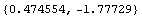
As expected, the relative location of the centroid, with respect to the section, has not changed.
In[220]:=Show[rotpp,Epilog->MarkPoint[sc]];
You calculate and mark the location of the centroid of the unconventional cross section that was introduced previously.
In[221]:=pc=PolygonCentroid[TriangleCoordinates[ptsIsection]]
Out[221]=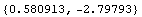
In[222]:=Show[tpIsection,Epilog->MarkPoint[pc]];
Here is the location of the centroid of the complex domain.
In[223]:=pc=PolygonCentroid[tcComplex]
Out[223]=
This shows the location of the centroid on the triangulation plot.
In[224]:=Show[tpComplex,Epilog->MarkPoint[pc]];
The centroid of a hand tool can be useful information. Compute the centroid of the wrench and mark it on its triangulation.
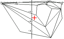
In[225]:=pc=PolygonCentroid[tcWrench]
Out[225]=
In[226]:=Show[tpWrench,Epilog->MarkPoint[pc]];
2.3.4 Moments of Inertia
The package NumCrossSectionProperties includes polygon versions of the moment functions that are examined in Section 2.2.4. The command ?*Moment* exhibits these correspondences.
In[227]:=
PolygonInertialMoments SectionInertialMoments
PolygonMomentsRotate SectionMomentsRotate
PolygonMomentsTranslate SectionMomentsTranslate
PolygonPolarInertialMoments SectionPolarInertialMoments
PolygonPolarMomentsRotate SectionPolarMomentsRotate
PolygonPolarMomentsTranslate SectionPolarMomentsTranslate


You calculate the moments of inertia of the T-section.
In[228]:=PolygonInertialMoments[tcSimple]
Out[228]=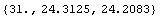
Find the moments of inertia of the unconventional T-section.
In[229]:=PolygonInertialMoments[tcTsection]
Out[229]=
Next give the moments of inertia of the unconventional I-section.
In[230]:=PolygonInertialMoments[tcIsection]
Out[230]=
Then calculate the moments of inertia of the complex domain with an opening.
In[231]:=PolygonInertialMoments[tcComplex]
Out[231]=
Finally, find the moments of inertia of the wrench profile.
In[232]:=PolygonInertialMoments[tcWrench]
Out[232]=
There are three ways to calculate the moments of inertia of a rotated polygon.
The first method is to use the function PolygonMomentsRotate.


In[233]:=PolygonMomentsRotate[tcTsection,/10]//N
Out[233]=
For the second method, rotate the polygon using the function PolygonRotate, and then compute the moments of inertia of this rotated polygon.
In[234]:=rottcTsection=TriangleCoordinates[PolygonRotate[ptsTsection,{0,0},N[/10]]];
In[235]:=PolygonInertialMoments[rottcTsection]
Out[235]=
Use PolygonMomentsRotate with the previously computed moments of inertia for the third method.
In[236]:=PolygonInertialMoments[tcTsection]
Out[236]=
In[237]:=PolygonMomentsRotate[%,N[/10]]
Out[237]=


In[238]:=PolygonMomentsTranslate[tcSimple,{0.1,-0.1}]
Out[238]=
You may obtain the same result by using the moments of inertia, area, and centroid that were previously calculated:  = 31. = 31.  , ,  = 24.3125 = 24.3125  , ,  = 24.2083 = 24.2083  , area = 6.5 , area = 6.5  , and centroid = {1.70 , and centroid = {1.70  , 1.43 , 1.43 }. }.
In[239]:=PolygonMomentsTranslate[{31.,24.3125,24.2083},6.5,{1.70513,1.4359},{0.1,-.1}]
Out[239]=
You use the following functions for triangulated sections in the same manner as their counterparts for domain names in the previous section. PolygonPolarInertialMoments calculates the polar moments of inertia from a triangulation of the polygon domain.


You use the function PolygonPolarInertialMomentsRotate to compute the polar moments of inertia of a rotated polygon from its triangulation.


You use the function PolygonPolarMomentsTranslate to compute the polar moments of inertia of a translated polygon from its triangulation.


2.3.5 Principal Axes
For a cross section specified by a polygon, there exists a coordinate system  in which the product moment of inertia vanishes. You can determine this coordinate system either by rotating the original coordinate system in which the product moment of inertia vanishes. You can determine this coordinate system either by rotating the original coordinate system  with its origin axis system located at the centroid of the cross section, or by rotating the cross section with respect to the same coordinate system (O x y). You use the function DomainPrincipalAxesDirections to calculate the orientations of the principal axes. with its origin axis system located at the centroid of the cross section, or by rotating the cross section with respect to the same coordinate system (O x y). You use the function DomainPrincipalAxesDirections to calculate the orientations of the principal axes.

These are the coordinates of points specifying a rotated T-section.
In[240]:=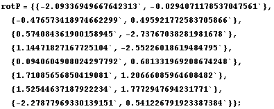
This shows the T-section.
In[241]:=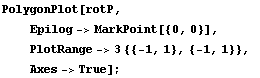
You can compute the orientations of the principal axes using the function PolygonPrincipalAxesDirections.
In[242]:=
Out[242]=
This shows that the centroid of the section is located at the origin of the coordinate system.
In[243]:=
Out[243]=
In[244]:=
Rotate the section by the orientations of the principal axes and calculate the moments of inertia. Note that the rotation angles are negated since it is the section that is rotated, not the coordinate systems.
In[245]:=
Out[245]=
In[246]:=
Out[246]=
|