|
Chapter 3
Bending of Cantilever Beams
3.1 Introduction
In designing engineering structures, such as buildings and bridges, cantilever beams are a main structural element receiving bending forces. This chapter considers the bending of a static cantilever beam of a constant cross section by a force at the end of the beam. The type of beam under consideration is also known as the Timoshenko beam due to the assumptions made in generating the equations of equilibrium for a beam. The analytical solutions are obtained by using the Saint-Venant's semi-inverse method. This stress function approach is adapted to obtain the stress and displacement distribution for various beam cross sections.
Structural Mechanics discusses closed-form solutions for the following set of beam cross sections:
 circular cross sections circular cross sections
 elliptical cross sections elliptical cross sections
 equilateral-triangular cross sections equilateral-triangular cross sections
 rectangular cross sections rectangular cross sections
For these cross sections, you can calculate the bending stress function, bending stresses, and the deflection of the center line of a beam. A number of two- and three-dimensional graphical functions are also available to generate illustrative representations of deflected beams under bending loads. For example, you can draw pictures of a cross section and a deflected beam by using the function CrossSectionPlot from the torsional analysis package TorsionAnalysis and the function BendingPlot from the BeamAnalysis package.
3.2 Circular Cross Section
Using the cross-section plotting function CrossSectionPlot, introduced in the torsional analysis package TorsionAnalysis, you can visualize a number of cross sections included in the package BeamAnalysis.


This shows a circle with a unit radius and a number of options for the Mathematica function Plot.
In[1]:=
In[2]:=
In[3]:=crsec=CrossSectionPlot[Domain[CircularSection,1],
AspectRatio->1,
PlotRange->{2{-1,1},2{-1,1}},
Axes->True,
Frame->True];
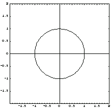
To simplify the equations of equilibrium of an elastic body under bending, the stress function, which may be viewed as a potential for the stress components, is introduced. BendingStressFunction calculates the stress function of various cross sections.


Compute the stress function for a circular shaft with radius  . The Poisson's ratio of the shaft material is . The Poisson's ratio of the shaft material is  , the moment of inertia about the y axis is , the moment of inertia about the y axis is  , and the applied force at the end of the shaft is P. The coordinate variables are x and y, respectively. , and the applied force at the end of the shaft is P. The coordinate variables are x and y, respectively.
In[4]:=
Out[4]=
You compute the moment of inertia about the y axis using the function SectionInertialMoments from the SymCrossSectionProperties package.
In[5]:=mm=SectionInertialMoments[CircularSection, ] ]
Out[5]=
Threading the replacement rule operator (->) over the symbols { , ,  , ,  } and the entries of mm, you generate a list of replacement rules for the moments of inertia terms. } and the entries of mm, you generate a list of replacement rules for the moments of inertia terms.
In[6]:=moi=Thread[{Ixx,Iyy,Ixy}->mm]
Out[6]=
Replacing the term  in the resulting stress function with the expression corresponding to this moment of inertia, you calculate the stress function in terms of (x, y), the Poisson's ratio of the shaft material, and the radius of the cross section. in the resulting stress function with the expression corresponding to this moment of inertia, you calculate the stress function in terms of (x, y), the Poisson's ratio of the shaft material, and the radius of the cross section.
In[7]:=
Out[7]=
The components of the stress tensor due to the bending force are calculated from the stress function associated with the cross section. Structural Mechanics has the function BendingStresses to calculate the bending stresses. Often, the x and y axes form the cross-section plane, and the x axis points downward. The z axis is the longitudinal axis of the cantilever beam (perpendicular to the cross-section plane). The root cross section is at z = 0.


In[8]:=
Out[8]=
Again, using the Mathematica function Thread, you generate a list of replacement rules for the stress components.
In[9]:=
Out[9]=
In[10]:=(stresscomponents=Thread[strnot-> Together[str]])//TableForm
Out[10]//TableForm=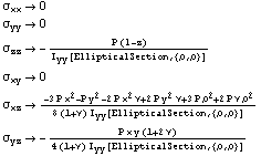
Replacing  in the equation with the previously calculated value for in the equation with the previously calculated value for  yields the stress components in terms of the parameters of this shaft model. yields the stress components in terms of the parameters of this shaft model.
In[11]:=
Out[11]//TableForm=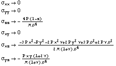
You can compute the deflection of the centerline of a cantilever beam under loading using the function CenterlineDeflection. The function calculates the deflection using a method based on the elementary theory of bending.


You can compute the centerline curve with no rotation and no displacement at the root section, that is, u'[0] == 0 and u[0] == 0.
In[12]:=
Out[12]=
Now you check that the boundary conditions, u'[0] == 0 and u[0] == 0, are really satisfied by this solution.
In[13]:=cen1/.z->0
Out[13]=
In[14]:=D[cen1,z]/.z->0
Out[14]=
As a numerical example, you use some values for the model parameters  , P, l, and , P, l, and  . .
In[15]:=
Out[15]=
The condition of no displacement at both the root section and at the midpoint of the shaft yields a different deflection curve.
In[16]:=
Out[16]=
You use the same numerical values for the model parameters.
In[17]:=
Out[17]=
In[18]:=
Out[18]=
Again, check that the boundary conditions are satisfied.
In[19]:=nc2/.z->0
Out[19]=
The slope of the centerline curve at the root section is nonzero in the case of this boundary condition.
In[20]:=D[nc2,z]/.z->0
Out[20]=
The second boundary condition is also satisfied.
In[21]:=nc2/.z->10/2
Out[21]=
The centerline curves for these two boundary conditions reveal the nature of the conditions. The line crossing the x axis at z = 5 corresponds to the condition u[0] == 0, u[l/2] == 0. The other line is obtained for the condition u'[0] == 0, u[0] == 0.
In[22]:=Plot[{u[z]/.nc1,u[z]/.nc2},{z,0,10}];

You use BendingPlot to generate a three-dimensional picture of a beam under bending.


The rotation of the beam cross section with respect to its centerline is defined for the shear modulus G.

The function BendingPlot defines the rotation with respect to the undeformed cross section, so you only use the second term in the previous expression for  , that is, , that is,  . .
First, you need to compute the coordinates of the vertices of a cross section. For the circular cross section, you calculate a table for the coordinates of 10 sampling points.
In[23]:=n=10;
cs=Table[ =2 =2 (i-1)/(n-1);{Cos[ (i-1)/(n-1);{Cos[ ],Sin[ ],Sin[ ]}//N,{i,1,n}]; ]}//N,{i,1,n}];
This shows the sampled cross section.
In[25]:=Show[Graphics[Line[cs]],AspectRatio->1];

You should calculate the rotation of the cross section from the components of the displacement vector. In this example, assume the rotation of the circular cross section is  . Note that the axis along the beam is z, the y axis is the horizontal axis, which is perpendicular to the beam cross section, and the horizontal axis is the x axis. . Note that the axis along the beam is z, the y axis is the horizontal axis, which is perpendicular to the beam cross section, and the horizontal axis is the x axis.
In[26]:=bp=BendingPlot[cs,u[z]/.nc1,z,- /20,10, /20,10,
PlotRange->{{0,12},{-3,3},{-3,3}},
PlotPoints->{Length[cs],15},
ViewPoint->{0.923,-3.216,0.508},
FaceGrids->{{-1,0,0},{0,1,0},{0,0,-1}},
AxesLabel->{z,y,x}];
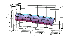
By choosing the command 3D ViewPoint Selector in the Input menu, you can set the ViewPoint option to a new value to show the deflected plot from a different angle. For example, you can view the deflected beam on the x-z plane by setting the ViewPoint option. Note that the Shading option is set to False.
In[27]:=Show[bp,ViewPoint->{-0.058,-3.382,0.104},Shading->False];
3.3 Elliptical Cross Section
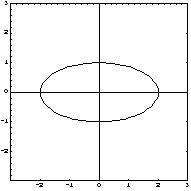
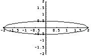
Consider the following elliptical cross section with radii of 2 units in length by 1 unit in height.
In[28]:=crsec=CrossSectionPlot[Domain[EllipticalSection,{2,1}],
AspectRatio->1,
PlotRange->{3{-1,1},3{-1,1}},
Axes->True,
Frame->True,
GridLines->None];
The most general form of the stress function for an elliptical cross section, with the radii ( , , ), the Poisson's ratio, and the moment of inertia about the y axis ), the Poisson's ratio, and the moment of inertia about the y axis , is calculated under the applied load P. , is calculated under the applied load P.
In[29]:=
Out[29]=
Here are the stress components for this cross section using the function BendingStresses.
In[30]:=
Out[30]=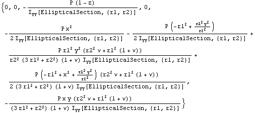
You calculate the moments of inertia for this section using the function SectionInertialMoments for the section object EllipseSector.
In[31]:=mm=SectionInertialMoments[EllipseSector,{r1,r2},{0,2 }] }]
Out[31]=
Threading the replacement rule operator (->) over the symbols { , ,  , ,  } and the entries of mm, you generate a list of replacement rules for the moment of inertia terms. } and the entries of mm, you generate a list of replacement rules for the moment of inertia terms.
In[32]:=moi=Thread[{Ixx,Iyy,Ixy}->mm]
Out[32]=
Next, replace the moment of inertia term in strs,  , with its value for the elliptical section, , with its value for the elliptical section,  . .
In[33]:=
Out[33]=
In[34]:=
Out[34]//TableForm=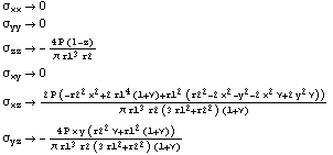
As in the case of the circular cross section, you first sample the ellipse, and then produce the plots of the deflected beam.
In[35]:=n=15;
cs=Table[ =2 =2 (i-1)/(n-1);{2Cos[ (i-1)/(n-1);{2Cos[ ],0.5Sin[ ],0.5Sin[ ]},{i,1,n}]//N; ]},{i,1,n}]//N;
Show[Graphics[Line[cs]],PlotRange->{{-2,2},{-2,2}},Axes->True ];
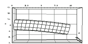
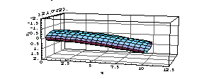
This shows the bent beam in a three-dimensional plot with a cross-section rotation of - /30. /30.
In[38]:=BendingPlot[cs,u[z]/.nc1,z,- /30,10, /30,10,
PlotRange->{{0,12.5},{-3,3},{-2,2}},
PlotPoints->{Length[cs],20},
ViewPoint->{0.923,-3.216,0.508},
FaceGrids->{{-1,0,0},{0,1,0},{0,0,-1}},
AxesLabel->{z,y,x}];
3.4 Rectangular Cross Section
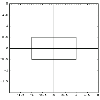
The domain name RectangularSection is used to specify a rectangular cross section. The cross section under consideration is specified by the coordinates of its vertices.
In[39]:=vertices={{1,1/2},{-1,1/2},{-1,-1/2},{1,-1/2},{1,1/2}};
In[40]:=CrossSectionPlot[vertices,
AspectRatio->1,
PlotRange->{2{-1,1},2{-1,1}} ,
Axes->True,
Frame->True,
PlotJoined->True,
GridLines->None];
The bending stress function in a rectangular section is expressed in series form. Mathematica 4 can express the sums in calculating the bending stress function in terms of hypergeometric functions. However, the output is a very long algebraic expression. To avoid the associated memory and CPU time problems, the Structural Mechanics function BendingStressFunction for RectangularSection returns the bending stress function in HoldForm. To evaluate the output, use the ReleaseHold function.
In[41]:=
In[42]:=
Out[42]=
Using functions in the package SymCrossSectionProperties, you can compute the moments of inertia for a rectangular cross section.
In[43]:=moi=SectionInertialMoments[RectangularSection,{-a/2,-b/2},a,b]
Out[43]=
The bending stress components in a rectangular section are expressed in series form.
In[44]:=
Out[44]=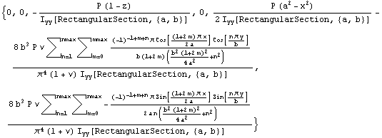
Here are the moments of inertia for this cross section.
In[45]:=moi=Thread[{Ixx,Iyy,Ixy}->moi]
Out[45]=
In[46]:=(strs=Thread[strnot->Together[str]])//TableForm
Out[46]//TableForm=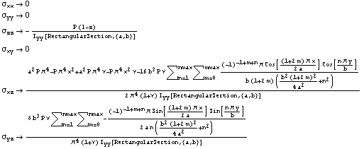
You replace the moment of inertia,  with its value in moi for the rectangular cross section. with its value in moi for the rectangular cross section.
In[47]:=
Out[47]//TableForm=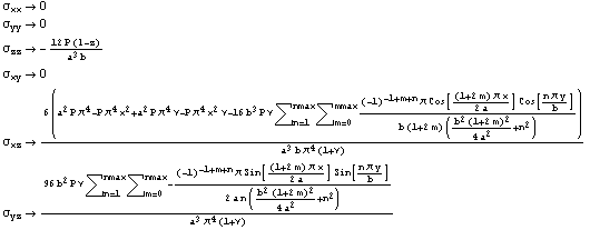
This computes the deflection of the centerline with a set of given boundary conditions u'[0] == 0 and u[0] == 0; it allows no deflection and no rotation for the cross section at z = 0.
In[48]:=
Out[48]=
In[49]:=Expand[cen[[1,2]]]
Out[49]=
Here you can verify that these two boundary conditions are satisfied.
In[50]:=D[cen[[1,2]],z]/.z->0
Out[50]=
In[51]:=cen[[1,2]]/.z->0
Out[51]=
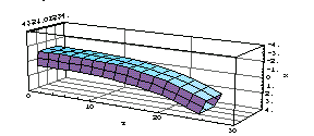
Now you can visualize the deflection of a rectangular cantilever beam for the deflection curve uz.
In[52]:=uz=.0001 z^2-.0002 z^3
Out[52]=
Create vertices of the cross section.
In[53]:=crossection=2{{1,1/2},{0,1/2},{-1,1/2},{-1,0},{-1,-1/2},
{0,-1/2},{1,-1/2},{1,0},{1,1/2}};
In[54]:=Show[Graphics[Line[crossection]],Axes->True];

Assume the rotation term  = =  at the point x = 0, y = 0. As previously noted, you can calculate the rotation using the following formula: at the point x = 0, y = 0. As previously noted, you can calculate the rotation using the following formula:

In[55]:=BendingPlot[crossection,uz,z,- /20,25, /20,25,
Boxed->True,
PlotRange->{{0,30},{-4,4},{-4,4}},
Axes->True,
PlotPoints->{Length[crossection],15},
Boxed->False,
FaceGrids->{{-1,0,0},{0,1,0},{0,0,-1}},
ViewPoint->{1.749, -2.792, 0.774},
AxesLabel->{z,y,x}];
3.5 Equilateral-Triangular Cross Section
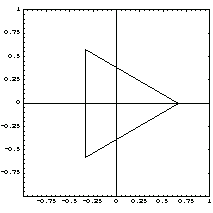
Here are the coordinates of the vertices of an equilateral-triangular cross section for the height a = 1 unit length.
In[56]:=vertices={{-a/3,-a/Sqrt[3]},{-a/3,a/Sqrt[3]},
{2a/3,0},{-a/3,-a/Sqrt[3]}}/.a->1;
You generate the shape of the cross section with CrossSectionPlot.
In[57]:=CrossSectionPlot[vertices,
AspectRatio->1,
PlotRange->{{-1,1},{-1,1}} ,
Axes->True,
Frame->True,
PlotJoined->True,
GridLines->None];
BendingPlot generates the three-dimensional plot of a bent equilateral-triangular beam. In order to avoid the torsional load due to a force applied at the tip of a beam, the force must be applied at the shear center of the cross section.
In[58]:=BendingPlot[vertices,4uz,z,- /15,10, /15,10,
Boxed->True,
PlotRange->{{0,12},{-2,2},{-2,2}},
Axes->True,
PlotPoints->{Length[vertices],20},
Boxed->False,
FaceGrids->{{-1,0,0},{0,1,0},{0,0,-1}},
ViewPoint->{1.749, -2.792, 0.774}];
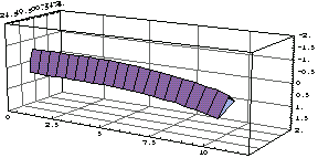
You obtain the stress function for a generic equilateral-triangular section using the domain object EquilateralTriangle in the function BendingStressFunction. Note that the bending function for the equilateral triangle is independent of Poisson's ratio  in the following computations. in the following computations.
In[59]:=
Out[59]=
You can generate the moments of inertia for the domain object EquilateralTriangle using the domain object RightTriangle for a = 1 unit length.
In[60]:=moi=(SectionInertialMoments[RightTriangle,{-a,0},3a,3a/2]+SectionInertialMoments[RightTriangle,{-a,0},3a,-3a/2])/.a->1
Out[60]=
In[61]:=moi=Thread[{Ixx,Iyy,Ixy}->moi]
Out[61]=
You can also compute the stress components in the beam by using BendingStresses for the cross-section object EquilateralTriangle.
In[62]:=
Out[62]=
In[63]:=strs=Thread[strnot->Together[str]]//TableForm
Out[63]//TableForm=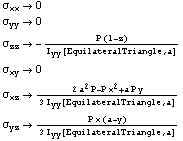
We replace the value of  with with  [ EquilateralTriangle, a ] in the stress components strs. [ EquilateralTriangle, a ] in the stress components strs.
In[64]:=
Out[64]//TableForm=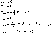
Here we compute the deflection of the centerline with a set of given boundary conditions.
In[65]:=
Out[65]=
|