|
Chapter 4
Torsional Analysis
4.1 Introduction
Because many engineering structures, such as beams, shafts, and airplane wings, are subjected to torsional forces, the torsional problem has been of practical importance in structural analysis for a long time. Saint-Venant (1885) was the first to provide the correct solution to the problem of torsion of bars subjected to moment couples at the ends. He made certain assumptions about the deformation of the twisted bar, and then showed that his solutions satisfied the equations of equlibrium and the boundary conditions. From the uniqueness of solutions of the elasticity equations, it follows that the assumed forms for the displacements are the exact solutions to the torsional problem. The technique adopted in Structural Mechanics is called the semi-inverse method.
Closed-form solutions of torsional problems exist for many cross sections. The purpose of this chapter is to present a set of known analytical solutions to the torsional problem. You can use the functions introduced in this chapter along with the built-in Mathematica functions as an interactive engineering handbook. Many examples and graphical representations of their solutions are also included.
The following types of cross sections are considered:
 circular cross sections circular cross sections
elliptical cross sections
rectangular cross sections
equilateral-triangular cross sections
sectorial-type cross sections
semicircular cross sections
For almost all these cross sections, functions for stress conditions, displacement components, stress components, twist per unit length, torsional rigidity, and warping functions are provided. The TorsionAnalysis package does not include the warping function and displacement components for the cross sector Sector due to the lack of closed-form expressions.
For shafts, only the following torsional rigidities are provided:
bar of narrow rectangular cross section
hollow concentric circular section
thin circular open tube of constant thickness
hollow (similar) elliptical cross section
4.2 Circular Cross Section
4.2.1 General Remarks
First, consider the torsion of a shaft with a circular cross section. Assume that the shaft is fixed at the origin of the Cartesian coordinate system. The z coordinate is along the shaft axis. Also note that units in this section are assumed to be consistent.
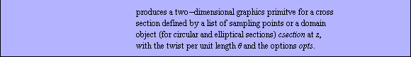
The domain name for a circular cross section is CircularSection. Draw a picture of a circular cross section with unit radius using the function CrossSectionPlot with some options.
In[1]:=
In[2]:=
In[3]:=
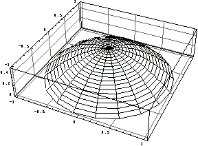
Use the function TorsionPlot to represent the rotation graphically. In the plots obtained by TorsionPlot, only the outer surfaces of solid shafts are shown unless it is noted that the cross section is hollow.

To rotate the (free) end cross section at z = 10 unit length by  /2 with respect to the cross section at the fixed end (at z = 0), the twist per unit length /2 with respect to the cross section at the fixed end (at z = 0), the twist per unit length  is (/2) (1/10). Now draw the shaft with this rotation. is (/2) (1/10). Now draw the shaft with this rotation.
In[4]:=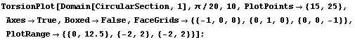
As indicated in its usage message, the options for TorsionPlot are the same as those for ParametricPlot3D.
Look at the rotation of the cross sections at the middle (z = 5) and at the end (z = 10) with respect to the root (at z = 0). The line from the origin of the axis system to the circles indicates the orientation of the root.

In[5]:=
In[6]:=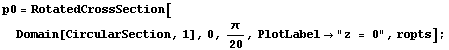
In[7]:=
In[8]:=
This shows how much each cross section is rotated with respect to its original position shown in the plot for the root section at z = 0.
In[9]:=
4.2.2 Torsional Analysis Functions for Circular Cross Sections
Using the function Twist, you can calculate the value of the applied moment in order to realize a specified amount of twist in a bar.

Calculate the twist per shaft length with a circular cross section.
In[10]:=
Out[10]=
You use the function TorsionalRigidity to calculate the torsional rigidity of a circular cross section, a commonly used design factor.

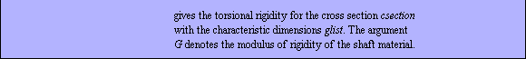
In[11]:=
Out[11]=
In the picture of the circular shaft, the value of is chosen to be (/2)(1/10). By replacing this in the twist relation and solving the resultant equation for the applied moment couple  , you can calculate the required applied moment for obtaining (/2)(1/10) twist per length. , you can calculate the required applied moment for obtaining (/2)(1/10) twist per length.
In[12]:=
Out[12]=
In[13]:=
Out[13]=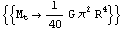
From this result, the applied moment is proportional to the fourth power of the shaft radius. If you double the shaft radius, the required applied moment for a specific rotation must be increased 16 times. So, in shaft design, the cross-section radius plays the most important role. You can generate the stress function for a circular cross section subjected to the torque  , with the radius , with the radius  , and the modulus of rigidity , and the modulus of rigidity  , by using the Mathematica function TorsionStressFunction. , by using the Mathematica function TorsionStressFunction.

In[14]:=
Out[14]=
Note that the stress function for a circular section is in Cartesian coordinates even though the cross section is circular.
Similarly, with the aid of the functions Displacements and Stresses, you can generate the displacement and stress components in terms of twist per length . In the following example, you can compute the three displacement components (u[x], u[y], u[z]), in the x, y, and z directions for CircularSection.

In[15]:=
Out[15]=
In this result, the displacement components seem independent of the shaft radius  . As shown earlier, the twist depends on the geometry, namely, the radius . As shown earlier, the twist depends on the geometry, namely, the radius  . The elastic properties of the shaft material, the modulus of rigidity . The elastic properties of the shaft material, the modulus of rigidity  , and the applied moment couple , and the applied moment couple  . .
In[16]:=
Out[16]=
By replacing the twist in the displacements disp, the displacement components are represented in terms of the geometry, the modulus of rigidity, and the applied moment couple.
In[17]:=
Out[17]=
In[18]:=
Out[18]=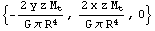
In[19]:=
Out[19]=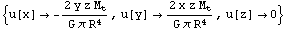
Similarly, compute the stress components as follows.

In[20]:=
Out[20]=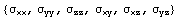
In[21]:=
Out[21]=
In[22]:=
Out[22]//TableForm=
Here the subscripts of  refer to the specific component of the stress tensor. The stress components are represented in terms of the geometry, the modulus of rigidity of the shaft material, and the applied moment couple. refer to the specific component of the stress tensor. The stress components are represented in terms of the geometry, the modulus of rigidity of the shaft material, and the applied moment couple.
In[23]:=
Out[23]//TableForm=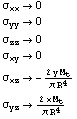
The nonzero stress components are inversely proportional to the fourth power of the radius of their shaft cross section. Thus, in shaft design, the diameter of the shaft plays a more important role than the modulus of rigidity. Clearly, the maximum stress values are realized on the lateral surface of the shaft.
In[24]:=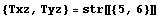
Out[24]=
In[25]:=
Out[25]=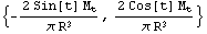
To represent the displacement field, use the function PlotVectorField from Graphics`PlotField` in the Mathematica 4 Standard Add-on Packages.
First, load the standard package PlotField.
In[26]:=
In[27]:=
Out[27]=
This gives the torsion stress function in polar coordinates.
In[28]:=
Out[28]=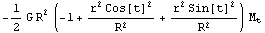
In[29]:=
This calculates the displacement field at z = 1 unit length for the radius r = 1 unit length and the applied torque M = 2 units.
In[30]:=
Out[30]=
In[31]:=
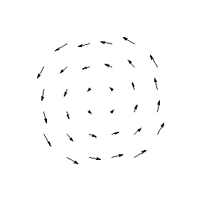
This shows the displacement field.
In[32]:=
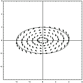
You can superimpose this vector field and the circular cross section obtained earlier.
In[33]:=
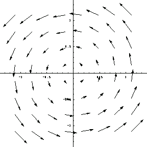
You can draw the displacement field using PlotVectorField as another way to represent the vector field.
In[34]:=
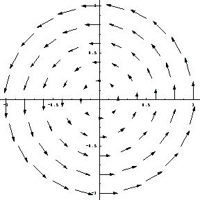
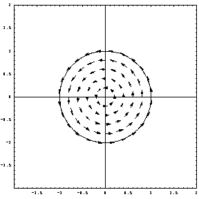
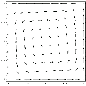
Since the cross section is circular, the vector field in the circular area is of interest. In the following, you develop a "mask" to cover the outside of this circular area. The bounding circle polylist is sampled at 20 points, and an outside frame is specifed by the list of points add. By assigning GrayLevel[1] to the area defined by this polygon, you obtain an invisible mask. When this mask is superimposed on top of a vector field, only the circular part of the vector field, which is the inside of the mask, will be visible.
In[35]:=
In[36]:=
In[37]:=
When the displacement vector field and this mask are superimposed, only the displacement field in the circular cross section is shown.
In[38]:=
From this result, you can see that the maximum values of displacements are realized at the circular boundary of the cross section. As seen in this vector field plot, due to the symmetry of the cross section, the displacement and stress fields are symmetric.
4.3 Elliptical Cross Section
4.3.1 General Remarks
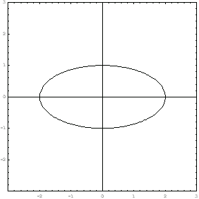
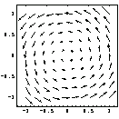
Consider a shaft with an elliptical cross section with the major axis 2a = 4 and the minor axis 2b = 2. Using the function CrossSectionPlot with the first argument EllipticalSection, you can obtain the drawing of the elliptical cross section.
In[39]:=
As in the circular cross-section problem, Structural Mechanics provides a number of functions for analysis of elliptical cross sections. These functions calculate the stress function, displacement and stress components, twist per unit length, torsional rigidity, and warping. Unlike the circular cross section, warping occurs in the shafts with elliptical cross sections due to the asymmetry.
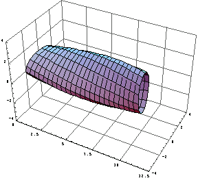
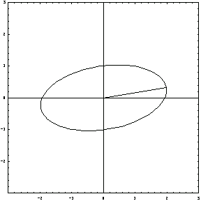
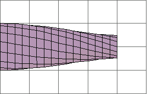
You plot a three-dimensional drawing of the twisted elliptical bar by using the function TorsionPlot with the cross-section object EllipticalSection. The argument list of this function indicates the shaft size and applied twist. The grids on the three background faces of the plot box are included with the option FaceGrids.
In[40]:=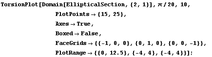
This shows the twisted cross section at z = 1. The line from the origin of the axis system to the ellipse boundary indicates the orientation of the root cross section.
In[41]:=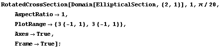
4.3.2 Torsional Analysis Functions for Elliptical Cross Sections
As in the case of the circular cross sections, you can obtain the twist per unit length and the torsional rigidity coefficient using the domain name EllipticalSection.
In[42]:=
Out[42]=
For  = =  , you get the twist for a circular cross section. , you get the twist for a circular cross section.
In[43]:=
Out[43]=
You compute the torsional rigidity for EllipticalSection.
In[44]:=
Out[44]=
Similarly, TorsionPlot generates three-dimensional plots of an elliptical cross section. However, by adjusting the option ViewPoint, you can obtain a two-dimensional view of the twisted cross section.
In[45]:=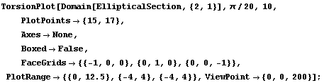
As calculated earlier, twist depends on geometry,  and and  , shaft material, , shaft material,  , and the applied moment couple, , and the applied moment couple,  . .
In[46]:=
Out[46]=
By replacing the twist in the displacements, you represent the displacement components in terms of the geometry, the modulus of rigidity of the shaft material, and the applied moment couple.
In[47]:=
Out[47]=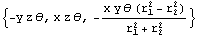
In[48]:=
Out[48]=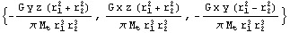
At z = 1, you calculate the x and y components of the displacement vector ( , ,  ) in the polar coordinates. ) in the polar coordinates.
In[49]:=
Out[49]=
You generate the displacement field for the major radius  = 2 units and minor radius = 2 units and minor radius  = 1 unit axes. = 1 unit axes.
In[50]:=
Out[50]=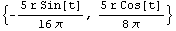
In[51]:=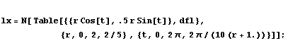
Using the function ListPlotVectorField from the standard package Graphics`PlotFields, you obtain a graphical representation of the displacement field.
In[52]:=
This shows how the vector field and the cross section look.
In[53]:=
Using TorsionalStresses, you generate the stress components in the bar due to the torsional load.
In[54]:=
Out[54]=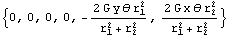
By replacing the twist , you get the displacement field in closed form in terms of the applied torque.
In[55]:=
Out[55]=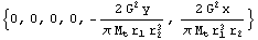
4.4 Rectangular Cross Section
4.4.1 General Remarks
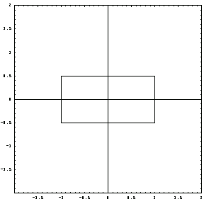
First, generate the graphical representation of the rectangular cross section using the coordinates of the vertices given in rsec.
In[56]:=rsec={{1,1/2},{-1,1/2},{-1,-1/2},{1,-1/2},{1,1/2}};
In[57]:=CrossSectionPlot[rsec,
PlotRange->2{{-1,1},{-1,1}},
Frame->True];
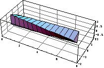
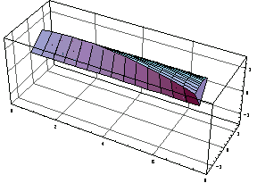
You can generate a 12-foot shaft under -/30 twist with the function TorsionPlot with a number of options.
In[58]:=TorsionPlot[rsec,-/30,12.,
PlotPoints->{5,15},
Axes->True,
Boxed->False,
FaceGrids->{{-1,0,0},{0,1,0},{0,0,-1}},
PlotRange->{{0,15},{-4,4},{-2,2}},
AxesLabel->{z,x,y}];

You can obtain additional lines representing the surface of the bar by including more sampling points in the cross section. For example, you use nine sampling points to represent the rectangular section.
In[59]:=
In[60]:=TorsionPlot[rsecnew,-/30,12.,
PlotPoints->{9,15},
Axes->True,
Boxed->False,
FaceGrids->{{-1,0,0},{0,1,0},{0,0,-1}},
PlotRange->{{0,15},{-4,4},{-2,2}},
AxesLabel->{z,x,y}
];
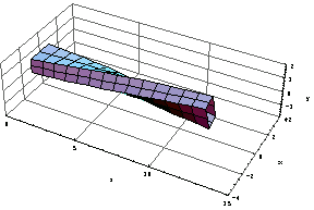
This shows how the section at z = 1 is rotated after the force is applied.
In[61]:=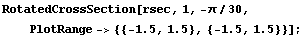
4.4.2 Torsional Analysis Functions for Rectangular Cross Sections
Here you can calculate the torsional rigidity of a rectangular cross section. The torsional rigidity for a rectangular section is expressed in series form.
In[62]:=
In[63]:=
Out[63]=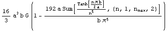
Similarly, you can obtain the twist per length for a rectangular cross section.
In[64]:=
Out[64]=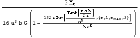
Roark's Formulas for Stress and Strain (p. 348, Table 20, Items 3 and 4) gives the torsional rigidity for a square cross section as 2.25  . Here you can compute the torsional rigidities for a square with the first 5 and 300 terms. Note that the series results converge rapidly. . Here you can compute the torsional rigidities for a square with the first 5 and 300 terms. Note that the series results converge rapidly.
In[65]:=N[TorsionalRigidity[RectangularSection,{a,a},G,{n,1,5}],20]
Out[65]=
In[66]:=N[TorsionalRigidity[RectangularSection,{a,a},G,{n,1,300}],20]
Out[66]=
The first four terms in this series expansion are computed symbolically.
In[67]:=TorsionalRigidity[RectangularSection,{a,b},G,{n,1,5}]//Expand
Out[67]=
Stress Fields
You compute the coefficient  in the relation in the relation 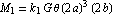 , introduced in Theory of Elasticity by Timoshenko and Goodier (p. 312), for various values of the ratio b/a. The first column rlist gives the values of the ratio b/a, and the second column klist gives the corresponding values of , introduced in Theory of Elasticity by Timoshenko and Goodier (p. 312), for various values of the ratio b/a. The first column rlist gives the values of the ratio b/a, and the second column klist gives the corresponding values of  . .
In[68]:=rlist={1,1.2,1.5,2.,2.5,3.,4.,5.,10,100,1000};
In[69]:=(k1list=Table[{rlist[[i]],N[TorsionalRigidity[RectangularSection,
{a,rlist[[i]] a},G,{n,1,255}]/(G (2a)^3 (2 rlist[[i]] a)),11]},
{i,1,Length[rlist]}])//TableForm
Out[69]//TableForm=
You compute the stress field by using the function TorsionalStresses with the first 5 terms and the domain name RectangularSection.
In[70]:=Clear[a,b]
In[71]:=(str=Thread[strnot->TorsionalStresses[RectangularSection,{1,1},1,1,{n,1,5},{x,y}]])//TableForm
Out[71]//TableForm=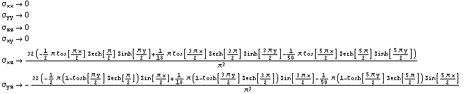
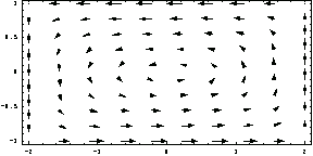
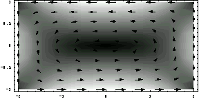
First you plot the traction field. The traction vector on the y-z plane consists of two components of the stress tensor,  and and  . .
In[72]:=
Using the traction field, visually examine the distribution of the magnitude of the traction on a surface of the twisted bar to determine stress concentrations. For example, from the following stress field, you could easily identify that the magnitude of the traction is maximum at the points (1, 0), (-1, 0), (0, 1), and (0, -1).
In[73]:=PlotVectorField[{Txz,Tyz}//N,{x,-1,1},{y,-1,1},
PlotPoints->10,
Frame->True];
Now consider the traction field for a rectangular section with a = 2 units length, b = 1 unit length. Consider the first 13 terms in calculating the stress components.
In[74]:=str=Thread[strnot->TorsionalStresses[RectangularSection,{2,1},1.,1.,{n,1,13},{x,y}]]//N;
In[75]:=
In[76]:=pv=PlotVectorField[{Txz,Tyz},{x,-2,2},{y,-1,1},
AspectRatio->1/2,
PlotPoints->10,
Frame->True,
AxesLabel->{"x","y"}];
You can also represent the magnitude of the traction using ContourPlot to visualize the traction intensity on a rectangular cross section. Create a contour plot of the traction field in the rectangular cross section.
In[77]:=
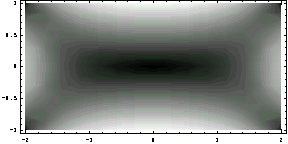
This shows the magnitude of the traction, cp, and the traction field, pv, on the same plot.
In[78]:=
From the above traction plot, observe that the maximum magnitudes occur at (0, 1) and (0, -1). Now compare these results obtained for G = 1 unit and = 1 radian against those reported in Timoshenko and Goodier's book (p. 312). In the following solution, consider the first 300 terms in the series solution for the stress components.
In[79]:=Clear[a,b,x,y]
In[80]:=str=Thread[strnot->TorsionalStresses[RectangularSection,{a,b},G,,{n,1,300},{x,y}]]//N;
In[81]:=
In the earlier numerical calculations, you saw that the maximum traction magnitude occurs at the point x = 0, y = ± b for  since since  = 0 at this point. As in the Timoshenko and Goodier's book (p. 312, eq. 166), you can compute the maximum stress value, = 0 at this point. As in the Timoshenko and Goodier's book (p. 312, eq. 166), you can compute the maximum stress value,  , for a square cross section. , for a square cross section.
In[82]:=Txz/.{b->a,x->0,y->-a}
Out[82]=
This is the distribution of the stress component  along the x axis (y = -1). along the x axis (y = -1).
In[83]:=Plot[Txz/.{a->1,b->1,y->-1,->1,G->1},{x,-1,1}];
Here you can plot how the stress component  varies in the cross section. varies in the cross section.
In[84]:=
Now compute the maximum traction on the surface for a number of rectangular cross sections: the maximum traction occurs at the points x = 0, y = ± b for a  b, and at the points x = ± a and y = 0 for b a. The first column is the ratio b/a and the second column is the corresponding value of k = b, and at the points x = ± a and y = 0 for b a. The first column is the ratio b/a and the second column is the corresponding value of k =  / (2 G a). / (2 G a).
Without loss of generality, fix a = 1 unit, x = 1.0, and y = 0.0, and choose b a.
In[85]:=a=1.0;
x=1.0;
y=0.0;
Calculate the stress components and the traction by taking the first 560 terms into account.
In[88]:=str=Thread[strnot->TorsionalStresses[RectangularSection,{a,b},1.,1.,{n,1,560},{x,y}]];
In[89]:=
The values for b are 1, 1.2, 1.5, 2., 2.5, 3., 4., 5., 10, 100, and 1000. You can use a few very high values of b in computations to examine the limit behavior of the solution.
In[90]:=rlist={1,1.2,1.5,2.,2.5,3.,4.,5.,10,100,1000};
In[91]:=klist=Table[{rlist[[i]],(N[Tyz]/.{a->1.,b->rlist[[i]],x->1.,y->0})/2.},
{i,1,Length[rlist]}];
In[92]:=N[klist,11]//TableForm
Out[92]//TableForm=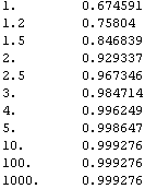
By recognizing  = k = k  from Eqs. 167 and 172 in Theory of Elasticity, you can easily generate the results in the table on page 312 for n = 255. from Eqs. 167 and 172 in Theory of Elasticity, you can easily generate the results in the table on page 312 for n = 255.
In[93]:=k1list=Table[{rlist[[i]],N[TorsionalRigidity[RectangularSection,{a,rlist[[i]] a},G,{n,1,255}]/(G(2a)^3 (2 rlist[[i]] a)),11]},{i,1,Length[rlist]}];
In[94]:=k1list//TableForm
Out[94]//TableForm=
In[95]:=N[{rlist,Transpose[klist][[2]],Transpose[k1list][[2]],Transpose[k1list][[2]]/Transpose[klist][[2]]},6]//Transpose//TableForm
Out[95]//TableForm=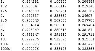
Compute the displacements by considering the first seven terms in the series solution.
In[96]:=Clear[x,y,z]
In[97]:=
Out[97]=
In[98]:=disp=Thread[dispnot->(TorsionalDisplacements[RectangularSection,{1,1},1,{n,1,7},{x,y,z}]/.z->1)]
Out[98]=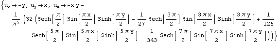
Here is the displacement field.
In[99]:=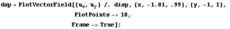
You can superimpose this field and the cross-section plot obtained with the function CrossSectionPlot.
In[100]:=crs=CrossSectionPlot[{{1,1},{-1,1},{-1,-1},{1,-1},{1,1}},
AspectRatio->1,
PlotRange->2{{-1,1},{-1,1}},
Frame->True,
Axes->None,
DisplayFunction->Identity];
In[101]:=Show[crs,dsp,DisplayFunction->$DisplayFunction];
From this displacement field, it is clear that the maximum displacements occur at the corners (1, 1), (1, -1), (-1, 1), and (-1, -1).
4.5 Equilateral-Triangular Cross Section
4.5.1 General Remarks
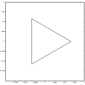
This section considers the stress and displacement distributions in an equilateral triangle. The coordinates of vertices of an equilateral triangle with height a are calculated.
In[102]:=points={{-a/3,-a/Sqrt[3]},{-a/3,a/Sqrt[3]},{2a/3,0},{-a/3,-a/Sqrt[3]}}/.a->1;
Here plot the shape of the cross section for a = 1.
In[103]:=

In[104]:=ss=CrossSectionPlot[points, PlotRange->{{-1,1},{-1,1}},
Frame->True ,DefaultFont->{"Courier",5},Axes->None];
Next, visualize this equilateral-triangular beam twisted by = /(4 ), where the beam length is ), where the beam length is  = 7. The end of the beam at z = 7 is rotated by /4 with respect to the root cross section at z = 0. = 7. The end of the beam at z = 7 is rotated by /4 with respect to the root cross section at z = 0.
In[105]:=TorsionPlot[points/.a->1,/28,7,
PlotPoints->{4,15},
FaceGrids->{{-1,0,0},{0,1,0},{0,0,-1}},
PlotRange->{{0,8},{-2,2},{-1,1}}];
4.5.2 Torsional Analysis Functions for Equilateral Triangles
You calculate the torsional rigidity of an equilateral-triangular cross section using the TorsionalRigidity function with the domain object EquilateralTriangle. The characteristic dimension of an equilateral-triangular cross section is its height.
In[106]:=Clear[a,G]
In[107]:=TorsionalRigidity[EquilateralTriangle,{a},G]
Out[107]=
To avoid replacing x, y, and z in the stress components, use the following replacements for only the right-hand side of the replacement rules.
In[108]:=str=TorsionalStresses[EquilateralTriangle,{a},G,,{x,y}]
Out[108]=
Calculate the stress components at x = -a / 3, y = 0.
In[109]:=str1=Thread[strnot->(str/.{x->-a/3,y->0})];
str1//TableForm
Out[110]//TableForm=
Calculate the stress field for a = 1 unit, G = 1 unit, and = 1 radian.
In[111]:=(str=Thread[strnot->TorsionalStresses[EquilateralTriangle,{1},1,1,{x,y}]])//TableForm
Out[111]//TableForm=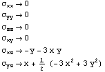
Next extract the traction components  , ,  from the stress tensor str. from the stress tensor str.
In[112]:=
Out[112]=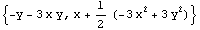
Now plot to see how the stress component  varies along the x axis from x = varies along the x axis from x =  to x = to x =  . .
In[113]:=
Similarly, you can obtain a plot showing how the value of  changes along the y axis. changes along the y axis.
In[114]:=
Here you can compute the stress distribution on the upper side of the cross sections. This gives the equation representing the upper edge of the triangle.
In[115]:=sol=Solve[{y==m x+ c/.{x->-a/3,y->a/Sqrt[3]},y==m x+ c/.{x->2a/3,y->0}},{m,c}]
Out[115]=
This is the replacement rule for the upper side.
In[116]:=upper=y->m x+ c/.sol[[1]]
Out[116]=
Compute the stress component Tyz along the upper side.
In[117]:=Tyz/.upper
Out[117]=
Now you can compute the magnitude of the traction along the upper surface of the cross section by plugging in the expression obtained earlier for this surface, here a = 1.
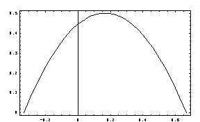
In[118]:=a=1.;
Plot[Evaluate[{Sqrt[Tyz^2+Txz^2]}/.upper],{x,-1/3,2/3},
PlotRange->All,
Frame->True,
AxesLabel->{"x"," "}];
ContourPlot is useful in representing the stress intensity. To draw contour lines in this triangular region, you can develop a mask that covers the outside of the triangular region. Set the gray-level primitive to 0 so that the contour lines are invisible outside of the cross section. Here are the vertices forming the mask.
In[120]:=
Out[120]=
In[121]:=add={{2,-.01},{2,-2},{-2,-2},{-2,2},{2,2},{2,-.01}}/2;
add={{points[[4]][[1]],-2},{-2,-2},{-2,2},{2,2},{2,-2},
{points[[4]][[1]],-2}}/2;
Use this mask to cover the contour lines that are outside of the cross section.
In[123]:=mask=Graphics[{GrayLevel[1],Polygon[Join[points,add]]}]
Out[123]=
Obtain the contour lines for the stress component  . .
In[124]:=sxz=ContourPlot[
Txz,{x,-1/3,2/3},{y,-1/Sqrt[3],1/Sqrt[3]},
Contours->50,
ContourShading->False];
Next plot the contour lines for the stress component  . .
In[125]:=syz=ContourPlot[
Tyz,{x,-1/3,2/3},{y,-1/Sqrt[3],1/Sqrt[3]},
Contours->50,
ContourShading->False];
Here are the contour lines for the stress component  inside the cross section. When printed, the displayed picture is a plain frame without the triangular part. inside the cross section. When printed, the displayed picture is a plain frame without the triangular part.
In[126]:=Show[sxz,mask, DisplayFunction->$DisplayFunction];
Plot the contour lines for the stress component  inside the cross section. inside the cross section.
In[127]:=Show[syz,mask];
Here are the contour lines for the magnitude of the traction on the x-y plane.
In[128]:=sVM=ContourPlot[
Sqrt[Tyz^2+Txz^2],{x,-1/3,2/3},{y,-1/Sqrt[3],1/Sqrt[3]},
PlotPoints->40,
Contours->40,
ContourShading->False];
Finally, you can obtain the contour lines for the magnitude of the traction on the x-y plane inside the cross section.
In[130]:=Show[sVM,mask];
4.6 Sector of a Circle and Semicircular Cross Sections
4.6.1 General Remarks
This section examines the torsional behavior of sectorial-type cross sections. The stress function for a general sector is given in series form. There is, however, an exact expression for the stress function for a semicircle, so a separate domain object is introduced for the semicircular domain SemiCircle. You can use the semicircle results to test the convergence of the series solution for sectorial cross section.
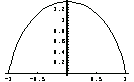
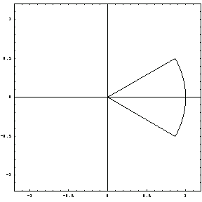
Here is a display of a circular sector originating at the center of the axis system with radius r = 1 and the sweeping angle  from -/3 to /3. from -/3 to /3.
In[131]:=crsec=CrossSectionPlot[
Domain[CircleSector,{0,0},1,{-/3,/3}/2],
Axes->True,
Frame->True,
PlotRange->1.2{{-1,1},{-1,1}}];
First, sample the boundary of the cross section so that you can employ TorsionPlot to display the twisted bar.
In[132]:==/3;
 =/(2*5); =/(2*5);
sli=Table[{Cos[ i],Sin[ i]},{i,-5,5}]//N;
sli=Join[{{0,0}},sli,{{0,0}}];
Here is a shaft of the previous cross section and a length of 7 units. The twist is /14 radian per unit length.
In[136]:=TorsionPlot[sli,/14,7.,
PlotPoints->{Length[sli],15},
Axes->True,
Boxed->True,
FaceGrids->{{-1,0,0},{0,1,0},{0,0,-1}},
PlotRange->{{0,8},{-1.5,1.5},{-1.5,1.5}}
];
4.6.2 Comparison of Results: SemiCircle versus CircleSector
The stress function of a general sector is expressed in series form, which is an approximation. However, there is an exact expression for the stress function for a semicircle. Due to the slow convergence of the series expressions in stress computations, this exact form for a semicircle is computationally efficient in many cases.
You can express the torsion stress function for a semicircle as follows.
In[137]:=Clear[r,G,,x,y]
In[138]:=TorsionStressFunction[SemiCircle,{r},G,,{x,y}]
Out[138]=
As a result of this form, you can compute the stress field in a semicircle in closed form.
In[139]:=str=TorsionalStresses[SemiCircle,{r},G,,{x,y}]
Out[139]=
Next, you numerically compare the results obtained using the function TorsionalStresses for CircleSector with = and SemiCircle. The geometric and material properties of the beam material are chosen as r = 1 unit, G = 1.1 units, and = 3.1 radians. It is worth noting that in the following the semicircle is defined by sweeping the polar angle from 0 to while the coordinate changes from -/2 to /2 in CircleSector. The domain name SemiCircle refers to the gray area. Also the domain representations are produced using the Mathematica graphics primitives, such as Disk and Text. You can also generate similar graphics with the help of the functions previously introduced .
In[140]:=$DefaultFont={"Courier", 8.};
In[141]:=opts={ AspectRatio->1,
Axes->True,
AxesFront->True,
Frame->True,
PlotRange->{{-1.1,1.1},{-1.1,1.1}},
AxesLabel->{"x"," "} };
In[142]:=Show[Graphics[{GrayLevel[0.70],Disk[{0,0},1,{0,}],
GrayLevel[0.0],
Text["O",{0.1,-0.10}],
Text["A",{0.99,-0.10}],
Text["B",{0.1,0.9}],
Text["C",{-0.99,-0.10}],
Disk[{0,0},0.03],
Disk[{1,0},0.03],
Disk[{0,1},0.03],
Disk[{-1,0},0.03]
}
], opts];
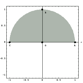
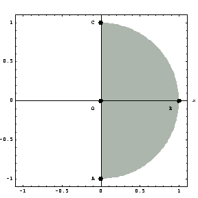
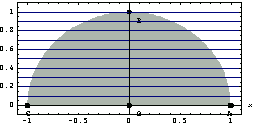
In the following plot, the semicircular cross section named CircleSector is depicted by the gray area.
In[143]:=Show[Graphics[{GrayLevel[0.70],Disk[{0,0},1,{-/2,/2}],
GrayLevel[0.0],
Text["O",{-0.1,-0.10}],
Text["A",{-0.10,-1.0}],
Text["B",{0.9,-0.1}],
Text["C",{-0.10,1.0}],
Disk[{0,0},0.03],
Disk[{1,0},0.03],
Disk[{0,1},0.03],
Disk[{0,-1},0.03]
}
],opts]
At the origin, point O where r = 0 and  = 0, you can compute the stress components using the first 40 terms in the series solution for the torsion stress function. = 0, you can compute the stress components using the first 40 terms in the series solution for the torsion stress function.
In[144]:=st=TorsionalStresses[CircleSector,{1,},1.1,3.1,{n,1,40},{0,10.^-5}]//N
Out[144]=
You use the Mathematica function Chop to eliminate the small quantities added to the solution due to numerical errors.
In[145]:=Thread[strnot->st//Chop]//TableForm
Out[145]//TableForm=
Using the domain object SemiCircle, compute the stress components at the origin. Note that the stress components and signs are different due to the locations of the two domains.
In[146]:=str=TorsionalStresses[SemiCircle,{1},1.1,3.1,{0,10^-5}]
Out[146]=
In[147]:=Thread[strnot->str]//TableForm
Out[147]//TableForm=
Compare the stresses at a point close to point A (at x = 0.99, y = 0.0 in the SemiCircle plot) computed by using the CircleSector and SemiCircle functions.
In[148]:=str=TorsionalStresses[SemiCircle,{1},1.1,3.1,{0.99,0.0}]
Out[148]=
In[149]:=Thread[strnot->str]//Chop//TableForm
Out[149]//TableForm=
Calculate the stress components close to point A (at x = 0.99, y = 0.0 in SemiCircle) using the CircleSector solution for the first 40 elements (n = 40).
In[150]:=st=TorsionalStresses[
CircleSector,{1,},1.1,3.1,{n,1,40},{0.0,-0.99}]//Chop//N
Out[150]=
This is the relative error for n = 40.
In[151]:=
Out[151]=
Calculate the stresses for n = 80 in this circular section.
In[152]:=
Out[152]=
Here is the relative error for n = 80.
In[153]:=
Out[153]=
You can improve the result substantially by doubling the number of terms in calculating stresses. Now increase n even more. Here are the stresses calculated with n = 160.
In[154]:=
Out[154]=
Calculate the relative error for n = 160.
In[155]:=
Out[155]=
Double the number of terms again to n = 320, and calculate the stress components.
In[156]:=
Out[156]=
This is the relative error for n = 320.
In[157]:=
Out[157]=
To illustrate the nature of the convergence of the series solution for stress components, you can generate a graph showing the relative error versus the number of terms plotted.
In[158]:=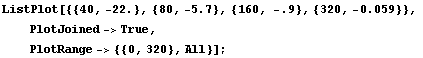
This graph clearly illustrates the benefit of being able to include more terms in torsional stress calculations. It is worth noting that Roark's Fomulas for Stress and Strain, one of the standard reference books in structural analysis, generally includes only the first four terms of the series solution in calculating the twist and maximum stress values for a large number of cross sections.
Next compare the two sets of stresses at a point close to point B ( x = 0, y = 0.99 in the SemiCircle plot).
In[159]:=str=TorsionalStresses[SemiCircle,{1},1.1,3.1,{0.0,0.99}];
Thread[strnot->str]//TableForm
Out[160]//TableForm=
In[161]:=TorsionalStresses[CircleSector,{1,},1.1,3.1,{n,1,50},{.99,0}]
Out[161]=
Finally, compare the stresses close to point C (x = -0.99 and y = 0) in the SemiCircle plot.
In[162]:=TorsionalStresses[CircleSector,{1,},1.1,3.1,{n,1,100},{0.0,.99}]
Out[162]=
In[163]:=str=TorsionalStresses[SemiCircle,{1},1.1,+3.1,{-.99,0.00}];
Thread[strnot->str]//TableForm
Out[164]//TableForm=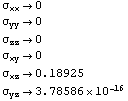
4.6.3 Applied Moments and Maximum Shearing Stresses in Sectors
The classic book Theory of Elasticity by S. P. Timoshenko and J. N. Goodier reports various values for the applied moment and for the maximum shearing stress along the circular and the radial boundaries of a number of sector sections. This section reproduces these results using functions from Structural Mechanics and provides results that are absent from their book.
The applied moment in terms of the torsional stress function can be expressed as
 = 2 = 2  r r (r, ) (r, )  r = k G r = k G
You can calculate the k values for various values by evaluating this integration for known G, , and a. Here are the values used in the computations.
In[165]:=={/4,/3,/2,2/3,,3/2,5/3,2}
Out[165]=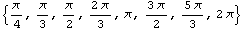
Take a = 1 unit length, G = 1 unit, and = 1 radian in the calculations for simplicity. These values for k were originally computed by Saint-Venant, later corrected by M. Aissen. Note that only the first 10 terms are considered here.
In[166]:=kvalues=Table[
int=TorsionStressFunction[CircleSector,{1,[[i]]+10^-6},1,1,{n,1,10},{r,}];
NIntegrate[2 int r,{r,0,1},{,-[[i]]/2+10^-6,[[i]]/2+10^-6}],{i,1,8}]
Out[166]=
You can express the maximum shearing stresses along the circular boundary as  G a. This maximum stress is realized at the point (a, 0) by taking G = 1 unit, a = 1 unit length, and = 1 radian. G a. This maximum stress is realized at the point (a, 0) by taking G = 1 unit, a = 1 unit length, and = 1 radian.
In[167]:=k1values=Table[
TorsionalStresses[CircleSector,{1,[[i]]+10^-6},1,1,{n,1,35},{1-10^-6,0}][[6]]//N,{i,1,8}]
Out[167]=
Unlike along the circular boundary, calculating the maximum shearing stresses along the radial boundary requires finding where these maximum values occur. To do this, define a dummy variable  for maximization. What you maximize here is the traction on the surface of a sector cross section. To use Mathematica's built-in minimization function FindMinimum, multiply the traction term by -1. You need to change the sign of the calculated maximum traction value after you perform minimization. for maximization. What you maximize here is the traction on the surface of a sector cross section. To use Mathematica's built-in minimization function FindMinimum, multiply the traction term by -1. You need to change the sign of the calculated maximum traction value after you perform minimization.
In[168]:=
In[169]:=k2=Table[alp=[[i]];
str=Take[ TorsionalStresses[
CircleSector,{1,alp+10^-6},1,1,{n,1,45},
{ro Cos[alp/2],ro Sin[alp/2]}]//N,-2];
FindMinimum[-Sqrt[str[[1]]^2+str[[2]]^2],{ro,.5}],{i,1,8} ]
Out[169]=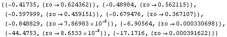
Extract and change the sign of the maximum traction values. Note that due to singularity, the maximum traction values for the section > /2 tend to  . .
In[170]:=k2values=Map[-#[[1]]&,k2]
Out[170]=
Represent the values of k,  , and , and  in tabular form. The first row gives the values of the sector cross sections, the second, third, and last rows are for k, in tabular form. The first row gives the values of the sector cross sections, the second, third, and last rows are for k,  , and , and  , respectively. , respectively.
In[171]:=TableForm[Partition[Transpose[{,kvalues,k1values,k2values}], 4], TableSpacing -> {1, 3}]
Out[171]//TableForm=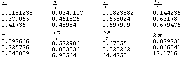
4.6.4 Stress Distribution in SemiCircle
Now calculate the stress component  profiles in a SemiCircle for r = 1 unit length at a number of station points along the y axis (y = 0.0, 0.2, 0.4, 0.6, 0.8, 1.0) as x varies from -1 to 1. profiles in a SemiCircle for r = 1 unit length at a number of station points along the y axis (y = 0.0, 0.2, 0.4, 0.6, 0.8, 1.0) as x varies from -1 to 1.
In[172]:=
In[173]:=
In[174]:=Show[Graphics[{GrayLevel[0.70],Disk[{0,0},1,{0,}],
GrayLevel[0.0],
Text["O",{0.1,-0.10}],
Text["A",{0.99,-0.10}],
Text["B",{0.1,0.9}],
Text["C",{-0.99,-0.10}],
Disk[{0,0},0.03],
Disk[{1,0},0.03],
Disk[{0,1},0.03],
Disk[{-1,0},0.03]
}
],opts];
In[175]:=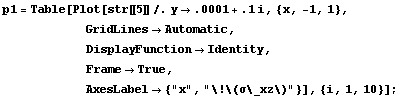
Now you can display how the value of  varies along these slicing lines. Note that you can identify the correspondence between the slicing lines and the following solution lines because the solutions are discontinous at the boundary of the cross section. varies along these slicing lines. Note that you can identify the correspondence between the slicing lines and the following solution lines because the solutions are discontinous at the boundary of the cross section.
In[176]:=Show[p1,DisplayFunction->$DisplayFunction];
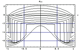
From this plot, you can conclude that the maximum  stress is realized at points A and C. stress is realized at points A and C.
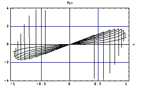
Next calculate the stress  in the same cross-section profiles at a number of station points along the y axis (y = 0.0 , 0.1, 0.2, ..., 0.9) as x varies from -1 to +1. in the same cross-section profiles at a number of station points along the y axis (y = 0.0 , 0.1, 0.2, ..., 0.9) as x varies from -1 to +1.
In[177]:=
Similarly, you can show how the value of  varies along these slicing lines. As noted earlier, you can identify the correspondence between the slicing lines and the following solution lines because the solutions are discontinous at the boundary of the cross section. varies along these slicing lines. As noted earlier, you can identify the correspondence between the slicing lines and the following solution lines because the solutions are discontinous at the boundary of the cross section.
In[178]:=Show[p1,DisplayFunction->$DisplayFunction];
4.7 Torsional Rigidities of Thin Tubes
Structural Mechanics includes the torsional rigidities for a number of well-known thin-walled cross sections. The domain objects for thin-walled sections are NarrowBar, HollowCircle, OpenHollowCircle, and HollowSimilarEllipse.
4.7.1 A Bar of a Narrow Rectangular Cross Section
Calculate the torsional rigidity of a narrow bar with modulus of rigidity, G, bar width, b, and bar thickness, c.
In[180]:=Clear[b,c,G,a]
In[181]:=TorsionalRigidity[NarrowBar,{b,c},G]
Out[181]=
You can verify this result by expanding the torsional rigidity of a thin bar that is found through the torsional rigidity of RectangularSection.
In[182]:=
Out[182]=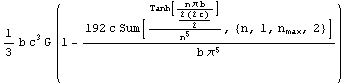
Since b is much larger than c, the ratio c/b is a very small number,  = c/b. = c/b.
In[183]:=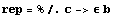
Out[183]=
Compute a series form solution by taking the first three terms of the expression rep, and expanding it around = 0.
In[184]:=
Out[184]=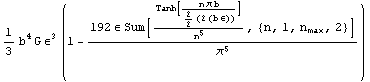
Since the term inside the first parentheses is order 1 for small , the torsional rigidity for a thin bar is  where stands for c/b. where stands for c/b.
In[185]:=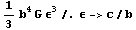
Out[185]=
4.7.2 Hollow Concentric Circular Sections
This section includes the torsional rigidity of a hollow concentric circular section whose outer radius and inner radii are  and and  , respectively. The modulus of rigidity of the shaft material is G. , respectively. The modulus of rigidity of the shaft material is G.
In[186]:=
Out[186]=
4.7.3 A Thin Circular Open Tube of Constant Thickness
Calculate the torsional rigidity for a thin circular open tube with a constant wall thickness t and median radius r. The modulus of rigidity of the shaft material is G.
In[187]:=TorsionalRigidity[OpenHollowCircle,{r,t},G]
Out[187]=
4.7.4 Hollow Cross Sections of Similar Ellipses
Similar ellipses are defined as  = =  / /  where where  and and  are the inner and outer major radii, and are the inner and outer major radii, and  and and  are the inner and outer minor radii of the hollow section. It is worth noting that the cross-section thickness is not constant for this cross section. are the inner and outer minor radii of the hollow section. It is worth noting that the cross-section thickness is not constant for this cross section.
In[188]:=
Out[188]=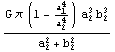
Note that the result is not a function of  since the ratio since the ratio  = =  / /  is constant. is constant.
4.8 Cross Sections of Complex Polynomial Stress Functions
4.8.1 General Remarks
The governing equation of torsion in the scaled-stress function accepts the function of complex variable as a solution. This section uses the solution to the following equation to examine a number of cross sections. as a solution. This section uses the solution to the following equation to examine a number of cross sections.
 + +  = 0 = 0
You can readily verify that the complex solution  satisfies this equation for every n. satisfies this equation for every n.
In[189]:=
Out[189]=
In[190]:=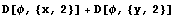
Out[190]=
The real and imaginary parts of this polynomial form a stress function and also satisfy the governing equation. Use the functions Re and Im from the package ReIm in the Mathematica 4 Standard Add-on Packages to extract the real and imaginary parts of the torsion function  . .
In[191]:=
In[193]:=
Out[193]=
In[194]:=
Out[194]=
You can calculate these real and imaginary stress functions for various values of n.
In[195]:=(tab1=Table[ex=Expand[(x+I y)^i];{Re[ex],Im[ex]},{i,1,7}])//TableForm
Out[195]//TableForm=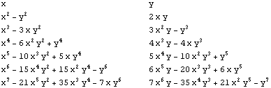
The first and second columns of this output correspond to the real and imaginary parts of a polynomial solution to the torsion equation.
4.8.2 Equilateral-Triangular Cross Sections
You can generate an equilateral-triangle-like cross section using the real part of the third-degree polynomial  - 3x - 3x  as given earlier. as given earlier.
In[196]:=tab1[[3,1]]
Out[196]=
Since the torsion function (x, y) is a scaled stress function, you need to add  to (x, y) to obtain the stress function. Calculate the stress function from the terms in the list tab1. to (x, y) to obtain the stress function. Calculate the stress function from the terms in the list tab1.
In[197]:=stressfunction=Factor[(1/2)(x^2+y^2)-(1/(2a)) tab1[[3,1]]+b]+c
Out[197]=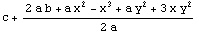
In[198]:=stressfunction=Factor[(stressfunction-c/.b->-2 a^2/27)]+c
Out[198]=
Various Cross Sections
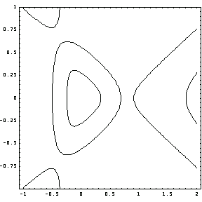
You can obtain various shapes of cross sections from this stress function by changing the value of the constant term c. In the following drawing, each cross section corresponds to a value of c.
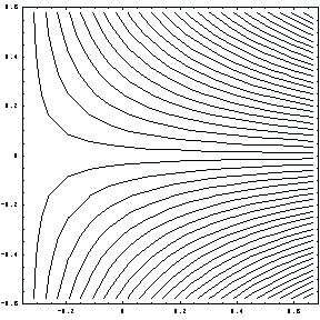
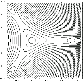
In[199]:=ContourPlot[
Evaluate[stressfunction/.c->0/.a->1],
{x,-1,2},{y,-2,2},
ContourShading->False,
Contours->5,
PlotRange->{-0.1,0.1},
PlotPoints->100];
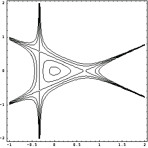
You can calculate the c value corresponding to a specific cross section from this plot. For the equilateral triangle, first read in the x and y coordinates of a point at the triangle. On a Macintosh computer, press the command key  and click (x, y) after selecting the plot. On all other computer platforms, find the instructions for reading coordinates of a point on a two-dimensional plot by choosing the menu item Get Graphics Coordinates under the Input menu of the tool bar. and click (x, y) after selecting the plot. On all other computer platforms, find the instructions for reading coordinates of a point on a two-dimensional plot by choosing the menu item Get Graphics Coordinates under the Input menu of the tool bar.
In[200]:={-0.354113, 0.588612}
Out[200]=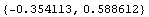
Using these coordinates, you can obtain the c value corresponding to this level curve.
In[201]:=cvalue=Solve[(Evaluate[stressfunction/.a->1]/.{x->-0.354113, y->0.588612})==0,c][[1,1,2]]
Out[201]=
Note that while the actual value of c for the level curve corresponding to the triangular cross section is 0, the computed cvalue is slightly smaller than zero due to reading inaccuracy by using Get Graphics Coordinates.
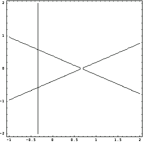
Now draw this cross section with one level curve.
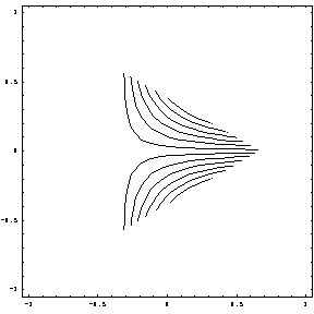
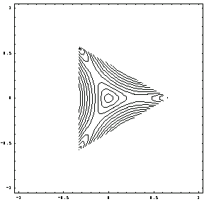
In[202]:=ContourPlot[Evaluate[stressfunction/.c->cvalue/.a->1],{x,-1,2},{y,-2,2},
ContourShading->False,
Contours->1,
PlotRange->{0,0},
PlotPoints->100];
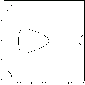
For the cross section that is the first closed curve inside the equilateral curve, you get the following.
In[203]:=cvalue=Solve[(Evaluate[stressfunction/.a->1]/.{x->-0.247368, y->0.043026})==0,c][[1,1,2]]
Out[203]=
In[204]:=segg=ContourPlot[Evaluate[stressfunction/.c->cvalue/.a->1],
{x,-1,2},{y,-2,2},
ContourShading->False,
Contours->1,
PlotRange->{0,0},
PlotPoints->100
];
Scaling Cross Sections
You can change the dimensions of a cross section, without changing its properties, by scaling the coordinates of the stress function. For example, if you double the height of the triangular cross section, the shape of the new cross section will still be equilateral.
In[205]:=ContourPlot[
Evaluate[stressfunction/.c->0/.a->1/.{x->(1/2)x,
y->(1/2)y}],{x,-1,2},{y,-2,2},
ContourShading->False,
Contours->1,
PlotRange->{-0.,0.},
PlotPoints->100];
Similarly, double the size of the egg-shaped cross section by rescaling the axes.
In[206]:=begg=ContourPlot[Evaluate[stressfunction/.
c->0.035/.a->1/.{x->(1/2)x,y->(1/2)y}],
{x,-1,2},{y,-2,2},
ContourShading->False,
Contours->1,
PlotRange->{-0.,0.},
PlotPoints->100];
Illustrate the two egg-shaped cross sections by superimposing their contour plots.
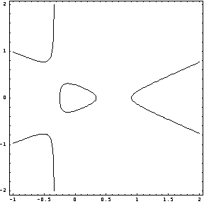
In[207]:=
Square-Like Cross Sections
To obtain the stress function for square-like cross sections, you can use the following combinations. Here the symbols a and c denote free parameters yet to be determined.
In[208]:=Clear[a,c,x,y];
stressfunction=(1/2)(x^2+y^2)-(a/2) tab1[[4,1]]+(a-1)/2+c
Out[209]=
You can calculate the values of the variable a that satisfy the boundary conditions for the stress function in terms of the coordinates of a point on the cross-section boundary. To do this, simply solve the stress function equation stressfunction = 0 for a. Note that the variable c is a free parameter to which you can set any value without violating the boundary conditions.
In[210]:=sol=Solve[stressfunction==0,a][[1]]
Out[210]=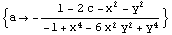
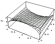
You can plot the surface defined by this solution for c = 0. Each level curve of this plot corresponds to a value for a and, consequently, a cross section associated with that particular a value
In[211]:=Plot3D[sol[[1,2]]/.c->0,{x,-.5,.5},{y,-.5,.5},
PlotPoints->30,
PlotRange->All];
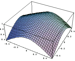
Draw five of these level curves (e.g., the cross sections) corresponding to the five values of a in the interval (-0.2, 0.2).
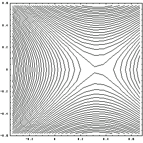
In[212]:=ContourPlot[sol[[1,2]]/.c->0,{x,-1,1},{y,-1,1},
ContourShading->False,
Contours->5,
PlotRange->{-.2,.2},
PlotPoints->60];
Likewise, use the 10 contour lines in the interval (0, 1.1) of the parameter a to generate the 10 corresponding cross sections.
In[213]:=ContourPlot[sol[[1,2]]/.c->0,{x,-1,1},{y,-1,1},
ContourShading->False,
Contours->10,
PlotRange->{0.,1.1},
PlotPoints->50];
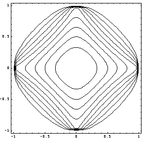
The value corresponding to a specific contour can be easily computed by replacing any coordinates in that contour into sol (for c = 0).
Here are two examples. First, read the coordinates of a point on each level curve for two curves.
In[214]:={-0.665084, 0.626658}
Out[214]=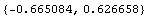
In[215]:={-0.315889, 0.031733}
Out[215]=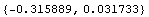
In[216]:=Solve[(stressfunction/.{x->-0.31, y->0.031626658}/.c->0)==0,a]
Out[216]=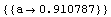
Then draw the level curve corresponding to a = 0.910788.
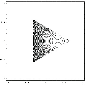
In[217]:=ContourPlot[sol[[1,2]]/.c->0,{x,-1,1},{y,-1,1},
ContourShading->False,
Contours->1,
PlotRange->{.910787,.910788},
PlotPoints->60
];
In[218]:=Solve[(stressfunction/.{x->-0.005493, y->-0.808921}/.c->0)==0,a]
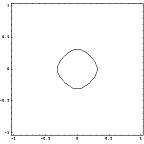
Out[218]=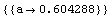
Here is the cross section for a = 0.604288.
In[219]:=ContourPlot[sol[[1,2]]/.c->0,{x,-1,1},{y,-1,1},
ContourShading->False,
Contours->1,
PlotRange->{.604288,.604289},
PlotPoints->60
];
|