Regulate an Inverted Pendulum
Regulate an Inverted Pendulum
In this classic control systems problem, a controller is designed to stabilize a system about an unstable equilibrium. The inverted pendulum is linearized about the vertical position. StateFeedbackGains gives a matrix, which can be thought of as a controller, that places the poles of the system in the left half of the complex plane. The closed-loop system is then simulated twice.
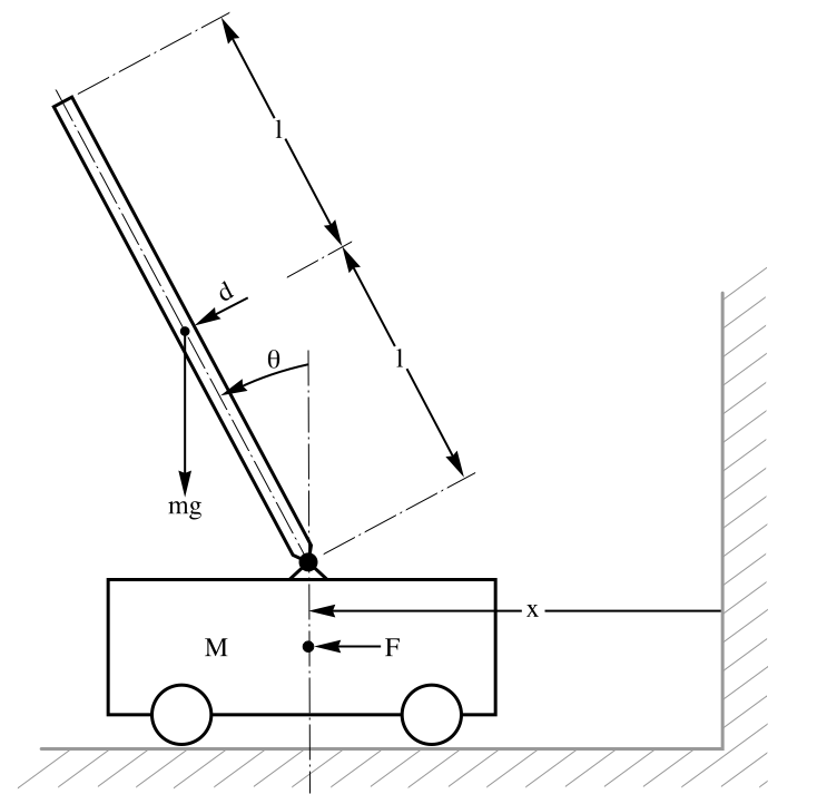
pendulum = StateSpaceModel[{(M + m)x''[t] - m l Sin[θ[t]] θ'[t]^2 + m l Cos[θ[t]] θ''[t] == F[t] + d[t] Cos[θ[t]], m x''[t] Cos[θ[t]] + m l θ''[t] == m g Sin[θ[t]] + d[t]}, {θ[t], θ'[t], x[t], x'[t]}, {F[t], d[t]}, {θ[t], x[t]}, t] /. {M -> 5.6, m -> 0.53, l -> 0.85, g -> 9.8};
poles = {-1 + 2I, -1 - 2I, -5, -7};k = Join[StateFeedbackGains[SystemsModelExtract[pendulum, 1], poles], {ConstantArray[0, 4]}]Plot[OutputResponse[{SystemsModelStateFeedbackConnect[pendulum, k], {0, 0.01, 0, 0}}, {0}, {t, 4}]//Evaluate, {t, 0, 4}, PlotRange -> All, PlotStyle -> {Blue, Red}, Epilog -> Inset[Column[{Style["x(t)", 10, Blue], Style["θ(t)", 10, Red]}], {3, 0.004}], AxesLabel -> {"t"}]Plot[OutputResponse[SystemsModelStateFeedbackConnect[pendulum, k], {0, UnitStep[t] - UnitStep[t - 1]}, {t, 4}]//Evaluate, {t, 0, 4}, PlotRange -> All, PlotStyle -> {Blue, Red}, Epilog -> Inset[Column[{Style["x(t)", 10, Blue], Style["θ(t)", 10, Red]}], {3, 0.5}], AxesLabel -> {"t"}]