Wolfram Language & System 13.2 (2022)|Legacy Documentation

This is documentation for an earlier version of Wolfram Language.View current documentation (Version 14)

BodePlot

BodePlot[lsys]

generates a Bode plot of a linear time-invariant system lsys.

BodePlot[lsys,{ω_min,ω_max}]

plots for the frequency range ω_min to ω_max.

BodePlot[expr,{ω,ω_min,ω_max}]

plots expr using the variable ω.

Details and Options

BodePlot plots the magnitude and phase of the transfer function of lsys.
The system lsys can be TransferFunctionModel or StateSpaceModel, including descriptor and delay systems.
For a system lsys with the corresponding transfer function , the following expressions are plotted:
continuous-time system

discrete-time system with sample time
BodePlot treats the variable ω as local, effectively using Block.
BodePlot has the same options as Plot, with the following changes and additions:

Exclusions	None	frequencies to exclude
FeedbackType	"Negative"	the feedback type
Frame	True	whether to draw a frame around each plot
MeshFunctions	{{#1&},{#1&}}	how to determine the placement of mesh divisions
PhaseRange	Automatic	range of phase values to use
PlotLayout	"VerticalGrid"	the layout to be used
PlotRange	{{Full,Automatic},{Full,Automatic}}	range of values to include
SamplingPeriod	None	the sampling period
ScalingFunctions	{{"Log10","dB"},{"Log10","Degree"}}	the scaling functions
StabilityMargins	False	whether to show the stability margins
StabilityMarginsStyle	Automatic	graphics directives to specify the style of the stability margins

Possible explicit settings for the option PlotLayout are "VerticalGrid" and "List".
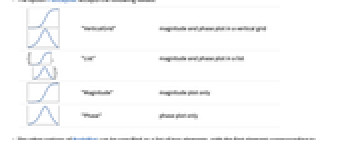
The option PlotLayout accepts the following values:

"VerticalGrid"

magnitude and phase plot in a vertical grid

{

}

"List"

magnitude and phase plot in a list

"Magnitude"

magnitude plot only

"Phase"

phase plot only

The other options of BodePlot can be specified as a list of two elements, with the first element corresponding to the magnitude plot and the second to the phase plot.
Option specifications include:

	opt->val	use val for both the magnitude and the phase plot
	opt->{val}	use val for the magnitude plot and the default for the phase plot
	opt->{val₁,val₂}	use val₁ for the magnitude plot and val₂ for the phase plot
	opt->{Automatic,val}	use the default for the magnitude plot and val for the phase plot

With the PlotLayout settings "Magnitude" or "Phase", a single setting refers to the plot requested.
The scaling functions can be specified as ScalingFunctions->{{magfreqscale,magscale},{phasefreqscale,phasescale}}.
The frequency scales magfreqscale and phasefreqscale can be "Log10" or "Linear", which correspond to the base-10 logarithmic scale and linear scale, respectively.
The magnitude scale magscale can be "dB" or "Absolute", which correspond to the decibel and absolute values of the magnitude, respectively.
The phase scale phasescale can be "Degree" or "Radian".

Examples

open allclose all

Basic Examples (3)

The Bode plot of a system:

A second-order system:

Plot over an explicit frequency range:

Bode plot of a state-space model:

Scope (13)

Bode plot of a constant-gain system:

Bode plot of an integrator:

Bode plot of a differentiator:

Bode plot of a first-order lag:

Bode plot of a first-order lead:

Bode plot of a second-order system:

A higher-order TransferFunctionModel:

Bode plot of a time-delay system:

A discrete-time system:

Specify the frequency range:

The Bode plot of a state-space model:

A system specified using its sinusoidal transfer function:

The Bode plot of a multiple-input, multiple-output system:

Generalizations & Extensions (1)

BodePlot[TransferFunctionModel[g,var]] is equivalent to BodePlot[g]:

Options (21)

CoordinatesToolOptions (5)

To obtain coordinates, select the graphics and press the period key:

If frequency is in rad/s, obtain coordinate frequency values in hertz by dividing it by :

Coordinate frequency values in different units for each plot:

Frequency values in original units, magnitude in absolute units, and phase in radians:

Specify radians as both the displayed and copied value of phase:

GridLines (3)

Show grid lines:

Show grid lines only on the magnitude plot:

Show specific grid lines:

GridLinesStyle (2)

Specify grid lines style:

Specify different grid lines styles:

PhaseRange (1)

The phase is typically plotted as a continuous function:

Specify a phase range:

PlotLayout (1)

By default, the magnitude plot is placed vertically above the phase plot:

Obtain the result in a list:

Only the magnitude plot:

Only the phase plot:

PlotTheme (2)

Use a theme with simple ticks and grid lines in a bright color scheme:

Change the color scheme:

SamplingPeriod (2)

Specify the sampling period in the system description:

Specify the sampling period in the BodePlot function:

A smaller sampling period results in a higher bandwidth:

ScalingFunctions (2)

Show absolute values of magnitude and phase in radians:

Plot frequency in the linear scale:

StabilityMargins (2)

Show stability margins:

Show the phase margin only:

StabilityMarginsStyle (1)

Specify the stability margins style:

Applications (7)

The static position error constant of a type 0 system is the magnitude at steady state:

Discrete-time type 0 system:

The static velocity error constant of a type 1 system is approximately the intersection of the initial dB/decade segment (or its extension) with the 0 dB line:

Discrete-time type 1 system:

The square root of the static acceleration error constant of a type 2 system is approximately the intersection of the initial dB/decade segment (or its extension) with the 0 dB line:

Discrete-time type 2 system:

Visualize the improvement in phase margin by using a proportional-integral (PI) compensator:

Visualize the frequency response of a zero-order hold with sampling period 1:

Obtain the Bode plot with frequency in Hertz, when the Laplace variable is in radians/second:

For continuous-time systems, the same result can be obtained by scaling the Laplace variable:

The plot in Hertz for a discrete-time system with the Z-transform variable in radians/second:

Properties & Relations (1)

SingularValuePlot generalizes the Bode magnitude plot to MIMO systems: