

ImageKeypoints
ImageKeypoints[image]
image の主な特徴を見付け出しその座標を返す.
ImageKeypoints[image,prop]
各特徴点について指定された特性 prop を返す.
ImageKeypoints[video,…]
video のフレーム中の特徴点を求める.
詳細とオプション
- 画像の特徴点は,形状,コントラスト,方向等の特定の画像の特徴をハイライトしている画像上の明確な位置のことである.対応する特徴点は,通常,画像の位置合せに使われる.
- ImageKeypoints[image]は画像の特徴点を見付け出し,その位置を{{x1,y1},{x2,y2},…}形式のリストとして返す.
- 指定可能な特性
-
"Confidence" ブロブ応答(正の数として与えられる) "ContrastSign" 特徴点が周囲より明るい場合は  ,その他の場合は

"Descriptor" 特徴点記述子 "Orientation" ラジアンで与えられた配向角 "OrientedDescriptor" 特徴点の配向記述子 "PixelPosition" 範囲  ,
 内の画素座標{x,y}
"Position" 範囲 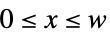 ,
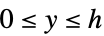 内の画像座標{x,y}
"Scale" 特徴点のスケール - ImageKeypointsは結果を特徴点の"Confidence"特性に基づいてソートする.
- ImageKeypoints[image,{prop1,prop2,…}]は複数の特性を返す.
- ImageKeypointsが返す特徴の記述子は平行移動,回転,スケール変更に対して数値的に強力である.
- 指定可能なオプション
-
KeypointStrength 0 特徴点の最小強度 Masking All 関心領域 MaxFeatures All 特徴点の最大数 Method "SURF" 返す特徴点のタイプ - MaxFeatures->n とすると,"Confidence"が最大で,最高で n 個の特徴点が返される.
- 使用可能なメソッド設定
-
"AGAST" 適応的かつ一般的なAccelerated Segment Test "AKAZE" Accelerated KAZEおよびバイナリ記述子 "BRISK" バイナリロバスト不変スケーラブル特徴点 "FAST" Accelerated Segment Testからの特徴 "KAZE" 非線形スケール空間ディテクタと記述子 "ORB" FASTディテクタとバイナリロバスト独立基本特徴(BRIEF) 記述子 "SIFT" スケール不変特徴変換検出器および記述子 "RootSIFT" 記述子が改善されたSIFTキーポイント "SURF" スピードアップしたロバストな特徴 - 指定したメソッドでは使えない特徴があるとき,結果中の対応する要素はMissing["NotAvailable"]に設定される. »
例題
すべて開く すべて閉じる例 (2)
スコープ (10)
ImageKeypoints[[image]]//ShortImageKeypoints[[image]]//ShortImageKeypoints[[image]]ImageKeypoints[[image], "Descriptor"]ImageKeypoints[[image], {"Scale", "Orientation", "ContrastSign"}]//MatrixForm特性"Position"と"PixelPosition"を得る:
pos = ImageKeypoints[[image], {"Position", "PixelPosition"}]pos[[All, 1]] + 1 / 2 == pos[[All, 2]]img = [image];scales = ImageKeypoints[img, "Scale"]特徴点の周りの真性領域のサイズに対応するスケール."SURF"特徴点の周りの円板領域を可視化する:
HighlightImage[img, {Thick, MapThread[Circle, {ImageKeypoints[img, "Position"], 2.5 * scales}]}, ImageSize -> 100]img = [image];orient = ImageKeypoints[img, "Orientation"]HighlightImage[img,
MapThread[
{Circle[#2, 5], Line[{#2, #2 + 5 * {Cos[#1], Sin[#1]}}]}&,
{orient, ImageKeypoints[img]}],
ImageSize -> 200]img = [image];
strength = ImageKeypoints[img, "Confidence"];
strength//ShortHistogram@strength特徴点の近傍の画素値の分布を表す"Descriptor"を得る:
img = [image];desc1 = ImageKeypoints[img, "Descriptor", MaxFeatures -> 1];desc2 = ImageKeypoints[ImageRotate@img, "Descriptor", MaxFeatures -> 1];EuclideanDistance[desc1, desc2]"ConstrastSign"は,周囲より明るい特徴点については1である:
ImageKeypoints[[image], "ContrastSign"]ImageKeypoints[[image], "ContrastSign"]オプション (11)
KeypointStrength (1)
Masking (1)
MaxFeatures (1)
Method (8)
i = [image];HighlightImage[i, ImageKeypoints[i]]HighlightImage[i, ImageKeypoints[i, Method -> "AKAZE", MaxFeatures -> 80]]"FAST"特徴点と"AGAST"特徴点は,スケール3.5における位置と強さで定義される:
i = [image];ImageKeypoints[i, {"Position", "Confidence", "Scale"}, Method -> "FAST", MaxFeatures -> 50]//ShortHighlightImage[i, ImageKeypoints[i, Method -> "FAST", MaxFeatures -> 50]]HighlightImage[i, ImageKeypoints[i, Method -> "AGAST", MaxFeatures -> 50]]"BRISK"特徴点と"ORB"特徴点は,その位置,スケール,方向,強さで定義される:
img = [image];{brisk, orb} = ImageKeypoints[img, {"Position", "Scale", "Orientation", "Confidence"}, Method -> #]& /@ {"BRISK", "ORB"};RandomSample[brisk, 2]RandomSample[orb, 2]記述子は0と1のベクトルで,"BRISK"については512,"ORB"については256である:
{brisk, orb} = ImageKeypoints[img, "Descriptor", Method -> #]& /@ {"BRISK", "ORB"};brisk[[1]]//Shortorb[[1]]//ShortDimensions[#]& /@ {brisk, orb}"AKAZE"特徴点と"KAZE"特徴点は,位置,スケール,方向,強さで定義される:
img = [image];{akaze, kaze} = ImageKeypoints[img, {"Position", "Scale", "Orientation", "Confidence"}, Method -> #]& /@ {"AKAZE", "KAZE"};RandomSample[akaze, 2]RandomSample[kaze, 2]ImageKeypoints[img, "Descriptor", Method -> "AKAZE"]//ShallowDimensions[%]KAZE記述子は単位ノルムの128個の実数のベクトルである:
ImageKeypoints[img, "Descriptor", Method -> "KAZE"]//Short{Dimensions[%], Norm /@ RandomSample[%, 5]}AKAZE配向記述子は,特徴点の固有配向についての補正なしで計算される:
img = [image];{kod, orientations} = Transpose@ImageKeypoints[img, {"OrientedDescriptor", "Orientation"}, Method -> "AKAZE"];δ = MapThread[HammingDistance, {kod, ImageKeypoints[img, "Descriptor", Method -> "AKAZE"]}];Pick[orientations, δ, x_ /; x < 20]"SURF"メソッドのとき,特徴点はその位置,スケール,方向,コントラストの符号,強さで定義される:
img = [image];surf = ImageKeypoints[img, {"Position", "Scale", "Orientation", "ContrastSign", "Confidence"}];RandomSample[surf, 2]SURF記述子は単位ノルムの64個の実数からなるベクトルからなる:
ImageKeypoints[img, "Descriptor", Method -> "SURF"]//Short{Dimensions[%], Norm /@ RandomSample[%, 5]}{kod, orientations} = Transpose@ImageKeypoints[img, {"OrientedDescriptor", "Orientation"}];δ = MapThread[EuclideanDistance, {kod, ImageKeypoints[img, "Descriptor"]}];Pick[orientations, δ, x_ /; x < 0.15]"SIFT"メソッドはスケール不変特徴変換を使って画像の特徴点の位置を求める:
img = [image];ImageKeypoints[img, {"Position", "Scale", "Orientation", "Confidence"}, Method -> "SIFT"];
RandomSample[%, 2]記述子は向きのヒストグラムを使って128個の数字のベクトルを構築する:
desc = ImageKeypoints[img, "Descriptor", Method -> "SIFT"];Short /@ RandomSample[desc, 2]Norm /@ RandomSample[desc, 5]"RootSIFT"メソッドは"SIFT"と同じ特徴点の位置とより改善された記述子を使う:
ImageKeypoints[[image], "Descriptor", Method -> "RootSIFT"]//ShortNorm /@ %//Shortアプリケーション (5)
スケール,方向,コントラストを使ってSURF特徴点を可視化する:
img = [image];
points = ImageKeypoints[img, {"Position", "Scale", "Orientation", "ContrastSign"}, MaxFeatures -> 100];
scalefactor = 2.5;
HighlightImage[img, Table[{{If[p[[4]] == 1, Yellow, Red], Circle[p[[1]], p[[2]] * scalefactor], Line[{p[[1]], p[[1]] + p[[2]] * scalefactor * {Cos[p[[3]]], Sin[p[[3]]]}}]}}, {p, points}]]img = [image];points = ImageKeypoints[img, {"Position", "Scale", "Orientation"}, Method -> "BRISK", MaxFeatures -> 50];
HighlightImage[img, {FaceForm[], Table[Rotate[{Line[{p[[1]], p[[1]] + p[[2]] * {1, 0}}], Rectangle[p[[1]] + p[[2]] * {-1, -1}, p[[1]] + p[[2]] * {1, 1}]}, p[[3]]], {p, points}]}]img = [image];
ImageTrim[img, {#}, 12]& /@ ImageKeypoints[img, Method -> "KAZE", MaxFeatures -> 100]{pos, size} = Transpose@ImageKeypoints[img, {"Position", "Scale"}, Method -> "KAZE", MaxFeatures -> 100];
MapThread[ImageTrim[img, {#1}, 2 * #2]&, {pos, size}]imgs = {[image], [image], [image]};
ImageTrim[#, ImageKeypoints[#, KeypointStrength -> .0005], 50]& /@ imgsImageCrop[ImageResize[#, {{240}, {180}}], {240, 180}]& /@ %10のカテゴリに属するそれぞれが32×32の5,000個の画像に「bag of words」を使ったオブジェクト認識:
obj = ResourceObject["CIFAR-10"];
training = ResourceData[obj, "TrainingData"];
testing = Flatten[Table[training[[i + 1000 ;; i + 1099]], {i, 1, 50000, 5000}]];training = Flatten[Table[training[[i ;; i + 499]], {i, 1, 50000, 5000}]];256×256画像について特徴点記述子を計算し,Visual Wordのコードブックを作る:
AbsoluteTiming[
	kp = ParallelTable[
	ImageKeypoints[ImageResize[i, 256], "Descriptor"], {i, training[[All, 1]]}
	];]
このコードブックには長さ64の画像記述子すべてが含まれている:
codebook = Flatten[kp, 1];
Dimensions[codebook]
AbsoluteTiming[
clust = ClusteringComponents[codebook, 100, 1, Method -> "KMeans", PerformanceGoal -> "Speed"];]codewords = Table[
p = Flatten@Position[clust, i];
Mean[codebook[[p]]],
{i, Max@clust}];画像の特徴はすべてのコード名の正規化された数として定義される:
nf = Nearest[codewords -> Automatic];imageCodewordsFeatureExtract[image_ ? ImageQ] := imageCodewordsFeatureExtract[ImageKeypoints[ImageResize[image, {256, 256}], "Descriptor"]];
imageCodewordsFeatureExtract[keypoints_List] := Module[
{h},
h = N@BinCounts[First@nf[#, 1] & /@ keypoints, {1, Length@codewords + 1}];
h / Total[h]
];imageCodewordsFeatureExtract[RandomSample[training][[1, 1]]]//Histogramt = Table[imageCodewordsFeatureExtract[kp[[i]]] -> training[[i, 2]],
{i, Length@training}];classifier = Classify[t];cm = ClassifierMeasurements[classifier, Table[imageCodewordsFeatureExtract[First@sample] -> Last@sample, {sample, testing}]];cm["ConfusionMatrixPlot"]特性と関係 (7)
すべてのメソッドですべての特性がサポートされている訳ではない:
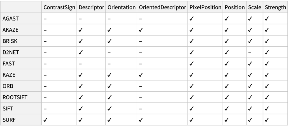
ある特性が指定されたメソッドでは使えないときは,Missing["NotAvailable"] が返される:
ImageKeypoints[[image], {"Position", "Descriptor"}, Method -> "FAST", MaxFeatures -> 5]ImageKeypoints[[image], {"Position", "ContrastSign"}, Method -> "AGAST", MaxFeatures -> 4]ImageKeypoints[[image], {"Position", "OrientedDescriptor"}, Method -> "BRISK", MaxFeatures -> 4]"SURF"記述子と"KAZE"記述子はユークリッド距離を使って比較されることが多い:
img = [image];kp = ImageKeypoints[img, {"Position", "Descriptor"}, MaxFeatures -> 11, Method -> "KAZE"];best = kp[[1, 2]];
distances = Table[EuclideanDistance[best, d], {d, kp[[2 ;; , 2]]}]"AKAZE","BRISK","ORB"の各記述子は,ハミング距離を使って比較されることが多い:
kp = ImageKeypoints[img, {"Position", "Descriptor"}, MaxFeatures -> 11, Method -> "BRISK"];best = kp[[1, 2]];
distances = Table[HammingDistance[best, d], {d, kp[[2 ;; , 2]]}]img = [image];
k = ImageKeypoints[img, {"Position", "Descriptor"}, MaxFeatures -> 80];
clust = FindClusters[k[[All, 2]] -> k[[All, 1]], 3];
colors = ColorData[3] /@ Range[Length[clust]];
HighlightImage[img, Transpose[{colors, clust}]]ImageCornersを特徴点として使うことができる:
img = [image];いくつかの特徴点記述子のスケールとの類似性のために,半径3.5でコーナーを計算する:
corners = ImageCorners[img, 3.5, MaxFeatureDisplacement -> 1, MaxFeatures -> 10]HighlightImage[img, {White, corners}]CornerFilterを使って検出されたコーナーの強さを得る:
cf = CornerFilter[img, 3.5];
strengths = ImageValue[cf, corners];
Transpose[{corners, strengths}]ImageKeypoints[img, {"Position", "Confidence"}, Method -> "FAST", MaxFeatures -> 10]ImageKeypoints[img, {"Position", "Confidence"}, Method -> "AGAST", MaxFeatures -> 10]ImageCorrespondingPointsはマッチする記述子を持つ特徴点の位置を与える:
{img1, img2} = {[image], [image]};{pos1, pos2} = ImageCorrespondingPoints[img1, img2];MapThread[HighlightImage, {{img1, img2}, {pos1, pos2}}]{k1, k2} = ImageKeypoints[#, {"Position", "Descriptor"}, MaxFeatures -> 100]& /@ {img1, img2};2番目の画像に対応する点があるものとないものの2つの特徴点を取る:
{m, n} = {k1[[23]], k1[[24]]};これらの特徴点についての記述子と2番目の画像中のすべての特徴点間のすべての距離を計算する:
δm = EuclideanDistance[m[[2]], #]& /@ k2[[All, 2]];
δn = EuclideanDistance[n[[2]], #]& /@ k2[[All, 2]];Histogram[#, ImageSize -> 200]& /@ {δm, δn}上位から2番目に近い比は,特徴点に対応点があるかどうかをみるために使われることが多い:
{bestm, secondbestm} = TakeSmallestBy[k2, EuclideanDistance[m[[2]], #[[2]]]&, 2];
{bestn, secondbestn} = TakeSmallestBy[k2, EuclideanDistance[n[[2]], #[[2]]]&, 2];EuclideanDistance[m[[2]], secondbestm[[2]]] / EuclideanDistance[m[[2]], bestm[[2]]]EuclideanDistance[n[[2]], secondbestn[[2]]] / EuclideanDistance[n[[2]], bestn[[2]]]{HighlightImage[img1, {Red, m[[1]], Yellow, n[[1]]}, ImageSize -> 250],
HighlightImage[img2, {White, k2[[All, 1]], Yellow, bestn[[1]], Red, bestm[[1]]}, ImageSize -> 250]}テキスト
Wolfram Research (2010), ImageKeypoints, Wolfram言語関数, https://reference.wolfram.com/language/ref/ImageKeypoints.html (2025年に更新).
CMS
Wolfram Language. 2010. "ImageKeypoints." Wolfram Language & System Documentation Center. Wolfram Research. Last Modified 2025. https://reference.wolfram.com/language/ref/ImageKeypoints.html.
APA
Wolfram Language. (2010). ImageKeypoints. Wolfram Language & System Documentation Center. Retrieved from https://reference.wolfram.com/language/ref/ImageKeypoints.html