
TimeSeriesAggregate
TimeSeriesAggregate[tes,dt]
重なり合ない幅 dt の窓上で,時系列または事象系列 tes の平均値を計算する.
TimeSeriesAggregate[tes,dt,f]
関数 f を,重なり合ない幅 dt の窓中の tes の値に適用する.
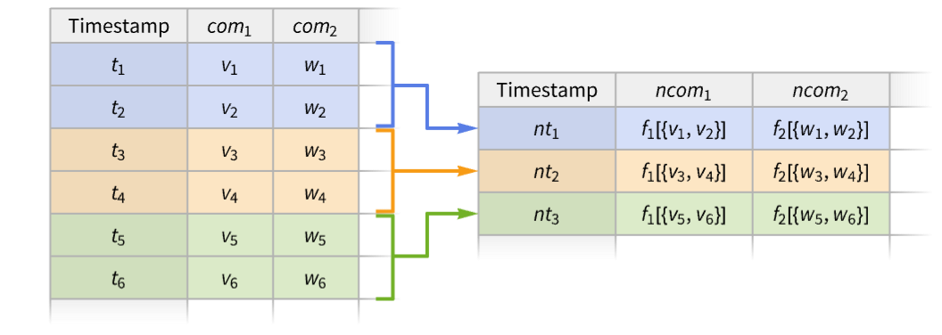
TimeSeriesAggregate[tes,dt,{ncom1f1,ncom2f2,…}]
関数 fiについて成分 ncomiを持つ新たな時(事象)系列を構築する.
詳細
- TimeSeriesAggregateは,年平均あるいは月の合計のような集約統計を計算するために,時(事象)系列解析にしばしば用いられる.
- TimeSeriesAggregateは,時(事象)系列 tes を,等幅(dt)の左が閉じて右が開いた不連続な窓に分割し,関数 f を各窓の値に適用する.
- 時(事象)軽鉄データ tes の可能な形式には以下がある.
-
TimeSeries[…] 連続時間順序付きサンプルデータ EventSeries[…] 値がある時間的事象の集合 TemporalData[…] 時点と値のペアからなる一つあるいは複数の経路 {{t1,x1},{t2,x2},…} 時点と値のペアのリスト {x1,x2,…} 0から始まる暗黙の整数時を持つ値のリスト - 窓に値がない場合,その窓は無視される.
- 窓の幅 dt は,正の数,Quantity,あるいは日付の増分として与えることができる.
- 窓指定 dt は,各窓内の新たなタイムスタンプの揃え方を指定する{dt,align}に拡張できる.
- 窓の揃え方 align の設定値には,Left,Center(デフォルト),Rightがある.
- 時(事象)系列 tes における構成要素"com"は,集約関数 f の引数として,構文 f[…,#com,…]&を用いて使用できる.
- 名前付きの構成要素を持たない単純な時系列に対しては,値は f[…,#,…]&または f[…,#Value,…]&のいずれかを用いてアクセスすることができる.
- TimeSeriesAggregateは,複数経路のTemporalDataオブジェクトについては,経路ごとに縫い込まれる.


例題
すべて開く すべて閉じる例 (3)
TimeSeries[{Subscript[x, 1], Subscript[x, 2], Subscript[x, 3], Subscript[x, 4], Subscript[x, 5], Subscript[x, 6]}, {1}]TimeSeriesAggregate[%, 2]Normal[%]TimeSeriesAggregate[{Subscript[x, 1], Subscript[x, 2], Subscript[x, 3], Subscript[x, 4], Subscript[x, 5], Subscript[x, 6]}, 2, Total]多成分時系列において,関数の引数として使用する値の成分を指定する:
ts = TimeSeries[{{11, "cat"}, {17, "dog"}, {13, "fox"}, {14, "cow"}, {10, "owl"}}, {0.}, {"a", "b"}];
Tabular[ts]TimeSeriesAggregate[ts, 3, {"max" -> (Max[#a]&), "joined" -> (StringJoin[#b]&)}]Tabular[%]スコープ (22)
基本的な用法 (5)
data = TimeSeries[{Subscript[x, 1], Subscript[x, 2], Subscript[x, 3], Subscript[x, 4], Subscript[x, 5]}, {1}]TimeSeriesAggregate[data, 2, f]%//Normaldata = RandomFunction[WienerProcess[], {0, 1, .01}]TimeSeriesAggregate[data, 0.05, Quantile[#, 95 / 100]&]ListLinePlot[{data, %}]data = TimeSeries[Accumulate@RandomReal[{-1, 1}, 250]]TimeSeriesAggregate[data, 10, Quartiles]Show[ListLinePlot[%], ListPlot[data, PlotStyle -> Gray]]data = FinancialData["GOOGL", {DateObject[{2019, 1, 1}, "Day"], DateObject[{2026, 1, 31}, "Day"]}]TimeSeriesAggregate[data, "Quarter", StandardDeviation]DateListPlot[%, GridLines -> {True, None}, PlotRange -> All]data = RandomFunction[BrownianBridgeProcess[{0, -1}, {2, 1}], {0, 2, .01}, 3]TimeSeriesAggregate[data, .15]Show[ListPlot[data], ListLinePlot[%, PlotStyle -> Thick]]データの型 (8)
関数 f を使って,4つずつのブロックにしたベクトルを合計する:
v = RandomInteger[{-10, 10}, 10]TimeSeriesAggregate[v, 4, f]data = {{"2005", 1}, {"2006", -1}, {"2007", 3}, {"2008", 6}, {"2009", -2}, {"2010", 4}, {"2011", 5}, {"2012", 4}, {"2013", 6}};TimeSeriesAggregate[data, {2, "Year"}]DateListPlot[{data, %}, PlotTheme -> "Detailed"]TimeSeriesの幅10の区間について,最大値を計算する:
ts = TimeSeries[TimeEventSeries`TimestampData[Association["UniformlySpacedQ" -> True, "Count" -> 100,
   "Endpoints" -> TabularColumn[Association["Data" -> {{0, 99}, {}, None},
      "ElementType" -> "Integer64"]], "MinimumTimeIncrement" -> 1, "Caller ...  -5.83329995009813, -5.365194518466113, -5.614668108914484,
      -6.477246191853266, -7.461704439607946, -6.79657593242878, -5.864937981765857,
-6.27785271209235, -5.841962111797332}, {}, None}, "ElementType" -> "Real64"]], Association[]];TimeSeriesAggregate[ts, 10, Max]ListLinePlot[{ts, %}]TemporalDataについて,幅10の中央値を計算する:
td = TemporalData[Automatic, {{{0.4948076687033609, -0.49167253739690864, -1.1692407506834863,
    -0.25256398166927063, -1.0324595217335713, -1.5365451139092143, -2.0662926057486564,
    -1.7443987109156156, -2.6969884040577115, -3.663349952028885, - ... 13,
    -5.365194518466113, -5.614668108914484, -6.477246191853266, -7.461704439607946,
    -6.79657593242878, -5.864937981765857, -6.27785271209235, -5.841962111797332}}, {{0, 99, 1}},
1, {"Discrete", 1}, {"Discrete", 1}, 1, {}}, False, 10.];TimeSeriesAggregate[td, 10, Median]ListLinePlot[{td, %}]EventSeriesについて,幅5の合計を計算する:
es = EventSeries[TimeEventSeries`TimestampData[Association["UniformlySpacedQ" -> True, "Count" -> 100,
   "Endpoints" -> TabularColumn[Association["Data" -> {{0, 99}, {}, None},
      "ElementType" -> "Integer64"]], "MinimumTimeIncrement" -> 1, "Calle ... 1, 1, 0, 1, 1, 0, 0, 0,
      0, 0, 0, 0, 0, 1, 0, 0, 0, 1, 1, 1, 0, 0, 0, 0, 0, 0, 1, 1, 0, 1, 0, 0, 1, 0, 1, 0, 1, 1, 1,
      0, 0, 1, 1, 1, 0, 0, 1, 1, 1, 1, 1, 0, 0, 0, 1, 1, 0}, {}, None},
"ElementType" -> "Integer64"]], Association[]];TimeSeriesAggregate[es, 5, Total]Show[ListLinePlot[%, InterpolationOrder -> 0], ListPlot[es, PlotStyle -> {Gray, AbsolutePointSize[3]}]]td = TemporalData[«4»];TimeSeriesAggregate[td, {6, "Month"}, Variance]DateListPlot[%, GridLines -> {Automatic, None}, PlotRange -> All, PlotLegends -> {"HP", "IBM"}]α = {{.2, .1}, {-.3, .2}};
β = {{.2, .5}, {-.2, .6}};
Σ = {{1, 0}, {0, .3}};
arima = RandomFunction[SARIMAProcess[{α}, 1, {}, {6, {β}, 1, {}}, Σ], {1, 10 ^ 3}]//TimeSeriesres = TimeSeriesAggregate[arima, 5, Map[Max[#] - Min[#]&, Transpose[#]]&]ListPointPlot3D[Table[Join[{t}, Normal[res[t]]], {t, 4, 998}], BoxRatios -> 1, ColorFunction -> Function[{t, x, y}, (ColorData["BlueGreenYellow"][t])], AxesLabel -> {"t", "x", "y"}]ts = TimeSeries[Quantity[{0, 16, 9, 3, 7, 2, 17, 10, 6, 12}, "Meters"]]TimeSeriesAggregate[ts, 2]ListLinePlot[{ts, %}, PlotLegends -> {"original time series", "aggregated time series"}, Filling -> Axis, AxesLabel -> Automatic]窓の幅 (5)
data = TimeSeries[{Subscript[x, 1], Subscript[x, 2], Subscript[x, 3], Subscript[x, 4]}, {1}]TimeSeriesAggregate[data, 2, f]//NormalTimeSeriesAggregate[data, {2, Center}, f]//Normaldata = FinancialData["APP", "2024"]TimeSeriesAggregate[data, Quantity[14, "Days"]];DateListPlot[{data, %}, GridLines -> {Automatic, None}]2四半期に渡るQuantity窓の平均:
data = FinancialData["GE", "2010"]TimeSeriesAggregate[data, Quantity[2, "QuarterYears"]]DateListPlot[{data, %}, GridLines -> {Automatic, None}]data = FinancialData["SBUX", "2020"]w = {{3, "Week"}, {2, "Day"}};TimeSeriesAggregate[data, w]DateListPlot[{data, %}, GridLines -> {Automatic, None}]data = FinancialData["SP500", "2020"]avg[w_] := TimeSeriesAggregate[data, w]wspec = {{1, "Week"}, {1, "Month"}, {1, "Quarter"}};Map[DateListPlot[avg[#], PlotLabel -> Last[#], ...]&, wspec]揃え (4)
data = TimeSeries[{Subscript[x, 1], Subscript[x, 2], Subscript[x, 3], Subscript[x, 4], Subscript[x, 5], Subscript[x, 6], Subscript[x, 7]}, {1}]TimeSeriesAggregate[data, {3, Center}, f]//NormalTimeSeriesAggregate[data, 3, f]//Normaldata = TimeSeries[{Subscript[x, 1], Subscript[x, 2], Subscript[x, 3], Subscript[x, 4], Subscript[x, 5], Subscript[x, 6], Subscript[x, 7]}, {1}]TimeSeriesAggregate[data, {3, Right}, f]//Normaldata = TimeSeries[{Subscript[x, 1], Subscript[x, 2], Subscript[x, 3], Subscript[x, 4], Subscript[x, 5], Subscript[x, 6], Subscript[x, 7]}, {1}]TimeSeriesAggregate[data, {3, Left}, f]//Normaldata = TimeSeries[Accumulate[RandomReal[{-1, 1}, 100]]]mavg = Table[TimeSeriesAggregate[data, {10, align}], {align, {Right, Center, Left}}];Equal@@(#["Values"]& /@ mavg)Equal@@(#["Times"]& /@ mavg)Show[ListPlot[data, PlotStyle -> Gray], ListLinePlot[mavg, PlotStyle -> Thick, PlotLegends -> {Right, Center, Left}]]アプリケーション (3)
出発 (1)
times = EntityValue[FlightData[Entity["Airport", "KORD"] -> All, "Flights", DateObject[{2022, 11, 11}]], "DepartureTime"];departures = EventSeries[1, {times}, TimeZone -> "America/Chicago"]res = TimeSeriesAggregate[departures, Quantity[1, "Hours"], Total]Show[DateHistogram[departures["Timestamps"], Quantity[1, "Hours"]], ListLinePlot[res]]労働人口 (1)
カリフォルニア州における労働人口の増加を,月ごとのデータに基づいて可視化する:
CAMonthlyLaborForce = EntityValue[...]growth = TimeSeriesAggregate[CAMonthlyLaborForce, {1, "Year"}]DateListPlot[growth, GridLines -> True, FrameLabel -> Automatic, PlotLabel -> "Annual average labor force in California"]市場のボラティリティ (1)
data = FinancialData["SP500", All]smooth = TimeSeriesAggregate[data, Quantity[5, "Years"], StandardDeviation];DateListPlot[smooth, PlotRange -> All, PlotTheme -> "Business"]smooth = TimeSeriesAggregate[data, Quantity[1, "Years"], InterquartileRange];DateListPlot[smooth, PlotRange -> All, PlotTheme -> "Business"]smooth = TimeSeriesAggregate[data, Quantity[2, "Years"], Max[#] - Min[#]&];DateListPlot[smooth, PlotRange -> All, PlotTheme -> "Business"]特性と関係 (1)
data = TimeSeries[{{0, a}, {1, b}, {2, c}}]left = TimeSeriesAggregate[data, {2, Left}, Total];
left//Normalcenter = TimeSeriesAggregate[data, {2, Center}, Total];
center//Normalright = TimeSeriesAggregate[data, {2, Right}, Total];
right//Normalテキスト
Wolfram Research (2014), TimeSeriesAggregate, Wolfram言語関数, https://reference.wolfram.com/language/ref/TimeSeriesAggregate.html (2026年に更新).
CMS
Wolfram Language. 2014. "TimeSeriesAggregate." Wolfram Language & System Documentation Center. Wolfram Research. Last Modified 2026. https://reference.wolfram.com/language/ref/TimeSeriesAggregate.html.
APA
Wolfram Language. (2014). TimeSeriesAggregate. Wolfram Language & System Documentation Center. Retrieved from https://reference.wolfram.com/language/ref/TimeSeriesAggregate.html