

WattsStrogatzGraphDistribution
WattsStrogatzGraphDistribution[n,p]
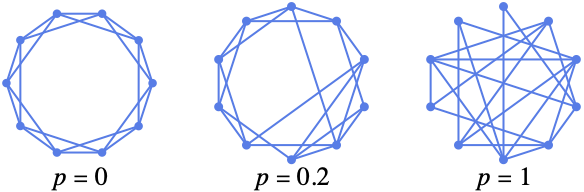
再配線確率が p で n 個の頂点を持つグラフのWatts–Strogatzグラフ分布を表す.
WattsStrogatzGraphDistribution[n,p,k]
再配線確率が p で2k 正則グラフから始まる n 個の頂点を持つグラフのWatts–Strogatzグラフ分布を表す.
詳細
- WattsStrogatzGraphDistributionは,スモールワールドグラフ分布としても知られている.
- WattsStrogatzGraphDistribution[n,p]はWattsStrogatzGraphDistribution[n,p,2]に等しい.
- WattsStrogatzGraphDistributionはCirculantGraph[n,Range[k]]から始まり各辺を確率 p で再配線することで構築される.各辺はループや多重辺を作らないように注意しながら1つの頂点を変更することで再配線される.
- WattsStrogatzGraphDistributionはRandomGraphやGraphPropertyDistribution等の関数で使うことができる.
例題
すべて開く すべて閉じる例 (2)
RandomGraph[WattsStrogatzGraphDistribution[50, 0.05]]再配線の確率の関数としてのGlobalClusteringCoefficient:
ListLogLinearPlot[Table[{p, GlobalClusteringCoefficient[RandomGraph[WattsStrogatzGraphDistribution[10 ^ 3, p, 5]]]}, {p, 10 ^ Range[-4, 0, 0.05]}], Joined -> True]スコープ (3)
RandomGraph[WattsStrogatzGraphDistribution[30, 0.03, 3]]RandomGraph[WattsStrogatzGraphDistribution[20, 0.07], 4]𝒟 = GraphPropertyDistribution[GlobalClusteringCoefficient[g], gWattsStrogatzGraphDistribution[10, 0.2]];NExpectation[x, x𝒟]アプリケーション (3)
Western States Power GridはWattsStrogatzGraphDistributionでモデル化することができる:
g = ExampleData[{"NetworkGraph", "PowerGrid"}];𝒢 = WattsStrogatzGraphDistribution[VertexCount[g], 0.25, Round[EdgeCount[g] / VertexCount[g]]]このモデルは,短い平均グラフ距離と高いクラスタリングで,経験的ネットワークというスモールワールドの特性を捉えている:
{N[MeanGraphDistance[g]], N[MeanClusteringCoefficient[g]]}h = RandomGraph[WattsStrogatzGraphDistribution[10 ^ 3, 0.25, 2]];{N[MeanGraphDistance[h]], N[MeanClusteringCoefficient[h]]}人口100人で住民1人あたりの知人の平均数が20人という小さい村のソーシャルネットワークはWattsStrogatzGraphDistributionでモデル化することができる.もっとも知人が少ない人の知人の期待数を求める:
𝒢 = WattsStrogatzGraphDistribution[100, 0.1, 20 / 2];g = RandomGraph[𝒢]𝒟 = GraphPropertyDistribution[Min[VertexDegree[h]], h𝒢];
NExpectation[x, x𝒟]𝒟 = GraphPropertyDistribution[GraphDiameter[h], h𝒢];Round[N[Mean[𝒟]]]以下はソーシャルネットワーク内での感染症の拡散モデルの簡約版を表す.感染症は各段階で確率0.4で罹患者から感染しやすい隣人に伝染し,感染した患者には回復後は免疫がある:
network = RandomGraph[WattsStrogatzGraphDistribution[100, 0.1, 3]]infect[z_, p_] := Pick[z, RandomChoice[{p, 1 - p} -> {1, 0}, Length[z]], 1];
step[g_, {i_, q_}, p_] :=
{Complement[infect[AdjacencyList[g, i], p], i, q], Join[q, i]};
infected[g_, i_, p_] := Last[FixedPoint[step[g, #, p]&, {i, {}}]]infected[network, {1}, 0.4] //ShortHighlightGraph[network, %]count[p_] := Mean[Table[Length[infected[network, {1}, p]], {100}]];DiscretePlot[count[p], {p, 0, 1, 0.1}, Joined -> True]特性と関係 (5)
GraphPropertyDistribution[VertexCount[g], gWattsStrogatzGraphDistribution[n, p, k]]GraphPropertyDistribution[EdgeCount[g], gWattsStrogatzGraphDistribution[n, p, k]]𝒟[n_, p_, k_] := HistogramDistribution[Flatten[Table[VertexDegree[g], {g, RandomGraph[WattsStrogatzGraphDistribution[n, p, k], 1000]}]], {-1 / 2, n, 1}];DiscretePlot[Evaluate@Table[PDF[𝒟[50, p, 2], d], {p, 0, 1, 1 / 3}], {d, 0, 8}, PlotRange -> All, ExtentSize -> 4 / 5]BinomialDistributionとPoissonDistributionの和による近似:
ℱ[n_, p_, k_] := TransformedDistribution[x + y, {xBinomialDistribution[2k, 1 - p / 2], yPoissonDistribution[k p]}]DiscretePlot[Evaluate@{PDF[𝒟[100, 0.4, 3], d], PDF[ℱ[100, 0.4, 3], d]}, {d, 0, 15}, PlotRange -> All, ExtentSize -> 4 / 5]ListLogLinearPlot[Table[{p, MeanGraphDistance[RandomGraph[WattsStrogatzGraphDistribution[10 ^ 3, p, 5]]]}, {p, Table[10 ^ x, {x, -3, 0, 0.3}]}], Joined -> True, PlotRange -> All]ListLogLinearPlot[Table[{p, GlobalClusteringCoefficient[RandomGraph[WattsStrogatzGraphDistribution[10 ^ 3, p, 5]]]}, {p, Table[10 ^ x, {x, -3, 0, 0.3}]}], Joined -> True]WattsStrogatzGraphDistribution[n,0,k]は 2k 正則グラフである:
RandomGraph[WattsStrogatzGraphDistribution[13, 0, 6]]VertexDegree[%]RandomGraph[WattsStrogatzGraphDistribution[12, 0, 6]]VertexDegree[%]テキスト
Wolfram Research (2010), WattsStrogatzGraphDistribution, Wolfram言語関数, https://reference.wolfram.com/language/ref/WattsStrogatzGraphDistribution.html.
CMS
Wolfram Language. 2010. "WattsStrogatzGraphDistribution." Wolfram Language & System Documentation Center. Wolfram Research. https://reference.wolfram.com/language/ref/WattsStrogatzGraphDistribution.html.
APA
Wolfram Language. (2010). WattsStrogatzGraphDistribution. Wolfram Language & System Documentation Center. Retrieved from https://reference.wolfram.com/language/ref/WattsStrogatzGraphDistribution.html