

WattsStrogatzGraphDistribution
WattsStrogatzGraphDistribution[n,p]
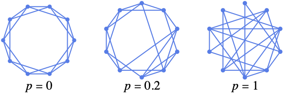
表示具有重连概率 p 的 n 顶点图的 Watts–Strogatz 图分布.
WattsStrogatzGraphDistribution[n,p,k]
表示起始于一个 2k 正则图,重连概率为 p 的 n 顶点图的 Watts–Strogatz 图分布.
更多信息
- WattsStrogatzGraphDistribution 亦称为小世界图分布.
- WattsStrogatzGraphDistribution[n,p] 等价于 WattsStrogatzGraphDistribution[n,p,2].
- WattsStrogatzGraphDistribution 构建于 CirculantGraph[n,Range[k]],且重连每条边的概率为 p. 通过改变一个顶点,重连每一条边,确保没有产生回路和创建多条边.
- WattsStrogatzGraphDistribution 可以与诸如 RandomGraph 和 GraphPropertyDistribution 等的函数一起使用.
范例
打开所有单元 关闭所有单元基本范例 (2)
RandomGraph[WattsStrogatzGraphDistribution[50, 0.05]]GlobalClusteringCoefficient 作为重连概率的函数:
ListLogLinearPlot[Table[{p, GlobalClusteringCoefficient[RandomGraph[WattsStrogatzGraphDistribution[10 ^ 3, p, 5]]]}, {p, 10 ^ Range[-4, 0, 0.05]}], Joined -> True]范围 (3)
RandomGraph[WattsStrogatzGraphDistribution[30, 0.03, 3]]RandomGraph[WattsStrogatzGraphDistribution[20, 0.07], 4]𝒟 = GraphPropertyDistribution[GlobalClusteringCoefficient[g], gWattsStrogatzGraphDistribution[10, 0.2]];NExpectation[x, x𝒟]应用 (3)
Western States Power Grid (西部各州电力网格)可以使用 WattsStrogatzGraphDistribution 建模:
g = ExampleData[{"NetworkGraph", "PowerGrid"}];𝒢 = WattsStrogatzGraphDistribution[VertexCount[g], 0.25, Round[EdgeCount[g] / VertexCount[g]]]在短均值图距离和高度集群下,该模型捕捉了经验网络的“小世界”特性:
{N[MeanGraphDistance[g]], N[MeanClusteringCoefficient[g]]}h = RandomGraph[WattsStrogatzGraphDistribution[10 ^ 3, 0.25, 2]];{N[MeanGraphDistance[h]], N[MeanClusteringCoefficient[h]]}下面是一个100人的村庄中的社交网络,其中每个人平均有20个关系,这个社交网络可以使用 WattsStrogatzGraphDistribution 建模. 求具有最少连接的人的期望关系数目:
𝒢 = WattsStrogatzGraphDistribution[100, 0.1, 20 / 2];g = RandomGraph[𝒢]𝒟 = GraphPropertyDistribution[Min[VertexDegree[h]], h𝒢];
NExpectation[x, x𝒟]𝒟 = GraphPropertyDistribution[GraphDiameter[h], h𝒢];Round[N[Mean[𝒟]]]这表示社交网络中传染性疾病传播的简化模型. 该疾病以每步概率 0.4 从受感染的人传播到周边易感人群,而受感染的人复原并且具有抵抗力:
network = RandomGraph[WattsStrogatzGraphDistribution[100, 0.1, 3]]infect[z_, p_] := Pick[z, RandomChoice[{p, 1 - p} -> {1, 0}, Length[z]], 1];
step[g_, {i_, q_}, p_] :=
{Complement[infect[AdjacencyList[g, i], p], i, q], Join[q, i]};
infected[g_, i_, p_] := Last[FixedPoint[step[g, #, p]&, {i, {}}]]infected[network, {1}, 0.4] //ShortHighlightGraph[network, %]count[p_] := Mean[Table[Length[infected[network, {1}, p]], {100}]];DiscretePlot[count[p], {p, 0, 1, 0.1}, Joined -> True]属性和关系 (5)
GraphPropertyDistribution[VertexCount[g], gWattsStrogatzGraphDistribution[n, p, k]]GraphPropertyDistribution[EdgeCount[g], gWattsStrogatzGraphDistribution[n, p, k]]𝒟[n_, p_, k_] := HistogramDistribution[Flatten[Table[VertexDegree[g], {g, RandomGraph[WattsStrogatzGraphDistribution[n, p, k], 1000]}]], {-1 / 2, n, 1}];DiscretePlot[Evaluate@Table[PDF[𝒟[50, p, 2], d], {p, 0, 1, 1 / 3}], {d, 0, 8}, PlotRange -> All, ExtentSize -> 4 / 5]使用 BinomialDistribution 和 PoissonDistribution 之和求近似:
ℱ[n_, p_, k_] := TransformedDistribution[x + y, {xBinomialDistribution[2k, 1 - p / 2], yPoissonDistribution[k p]}]DiscretePlot[Evaluate@{PDF[𝒟[100, 0.4, 3], d], PDF[ℱ[100, 0.4, 3], d]}, {d, 0, 15}, PlotRange -> All, ExtentSize -> 4 / 5]ListLogLinearPlot[Table[{p, MeanGraphDistance[RandomGraph[WattsStrogatzGraphDistribution[10 ^ 3, p, 5]]]}, {p, Table[10 ^ x, {x, -3, 0, 0.3}]}], Joined -> True, PlotRange -> All]ListLogLinearPlot[Table[{p, GlobalClusteringCoefficient[RandomGraph[WattsStrogatzGraphDistribution[10 ^ 3, p, 5]]]}, {p, Table[10 ^ x, {x, -3, 0, 0.3}]}], Joined -> True]WattsStrogatzGraphDistribution[n,0,k] 是一个 2k 正则图:
RandomGraph[WattsStrogatzGraphDistribution[13, 0, 6]]VertexDegree[%]RandomGraph[WattsStrogatzGraphDistribution[12, 0, 6]]VertexDegree[%]文本
Wolfram Research (2010),WattsStrogatzGraphDistribution,Wolfram 语言函数,https://reference.wolfram.com/language/ref/WattsStrogatzGraphDistribution.html.
CMS
Wolfram 语言. 2010. "WattsStrogatzGraphDistribution." Wolfram 语言与系统参考资料中心. Wolfram Research. https://reference.wolfram.com/language/ref/WattsStrogatzGraphDistribution.html.
APA
Wolfram 语言. (2010). WattsStrogatzGraphDistribution. Wolfram 语言与系统参考资料中心. 追溯自 https://reference.wolfram.com/language/ref/WattsStrogatzGraphDistribution.html 年