NDSolve::ndnco NDSolveValue::ndnco ParametricNDSolve::ndnco ParametricNDSolveValue::ndnco NDSolve`Reinitialize::ndnco
Examples
Basic Examples (4)
An error occurs because there are not enough initial conditions to uniquely specify a solution:
NDSolve[{f''[x] == f[x], f[0] == 1}, f, {x, 0, 1}]This shows a valid specification of a unique solution for this differential equation:
NDSolve[{f''[x] == f[x], f[0] == 1, f'[0] == 1}, f, {x, 0, 1}]This is a second-order ODE, but only one initial condition is given:
NDSolve[{(x / (1 + x)) D[y[x], {x, 2}] + ((2 x + 1) / (1 + x) ^ 2) D[y[x], {x, 1}] == 1 / (3 Sqrt[y[x]]), y[1] == 0}, y, {x, 1, 2}];A numerical solver needs more the one. This works, for instance:
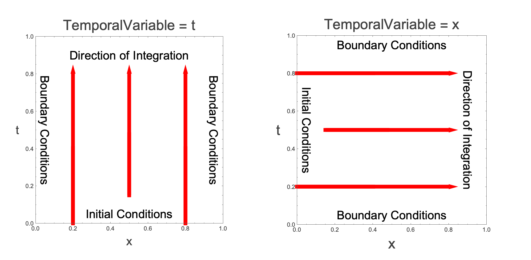
NDSolve[{(x / (1 + x)) D[y[x], {x, 2}] + ((2 x + 1) / (1 + x) ^ 2) D[y[x], {x, 1}] == 1 / (3 Sqrt[y[x]]), y[1] == 1, y'[1] == 0}, y, {x, 1, 2}]NDSolve[{D[u[x, t], {x, 2}] == D[u[x, t], {t, 2}], u[x, 0] == x * E ^ (-x ^ 2), Derivative[0, 1][u][x, 0] == 0, u[0, t] == 0}, u, {x, -10, 10}, {t, 0, 12}];For a numerical solution, you have to add a boundary condition. Refer to the picture below. Since there is an initial condition on the function and its first derivative at ![]() , the temporal variable is
, the temporal variable is ![]() . Therefore, boundary conditions are needed at
. Therefore, boundary conditions are needed at ![]() and
and ![]() . Two conditions are needed because the equation is second order in
. Two conditions are needed because the equation is second order in ![]() . Similarly, in the
. Similarly, in the ![]() -direction the equation is second order in
-direction the equation is second order in ![]() , so two conditions are needed. In the code above, there is just one boundary condition on
, so two conditions are needed. In the code above, there is just one boundary condition on ![]() at
at ![]() .
.
Adding the additional boundary condition resolves the error message:
NDSolve[{D[u[x, t], {x, 2}] == D[u[x, t], {t, 2}], u[x, 0] == x * E ^ (-x ^ 2), Derivative[0, 1][u][x, 0] == 0, u[0, t] == u[10, t] == 0}, u, {x, 0, 10}, {t, 0, 12}]Too many initial conditions are given here:
eqns = y''[r] + (Csch[r] - 1.25 Tanh[0.5 r] ^ 2) y'[r] + (-0.0005 Csch[0.5 r] ^ 2 Sech[0.5 r] ^ 4 (14 + 139 Cosh[r] - 30 Cosh[2 r] + 5 Cosh[3 r] + 32 Sinh[r] - 16 Sinh[2 r])) y[r] == 0;
conds = {y[0.01] == 0.01, y'[0.01] == 0.01, y[10] == 0.55, y'[10] == -0.3};
NDSolve[{eqns, conds}, y, {r, 0.01, 10}]
The problem is that too many conditions are given. The equation is a second-order ODE, so only two conditions on the function are needed:
conds2 = {y[0.01] == 0.01, y'[0.01] == 0.001};
sol2 = NDSolveValue[{eqns, conds2}, y, {r, 0.01, 10}]
However, the values at ![]() are not guaranteed to give
are not guaranteed to give ![]() ,
, ![]() as was stated in the original problem:
as was stated in the original problem:
{sol2[10], sol2'[10]}The solution is uniquely determined by the two initial conditions. Different initial conditions will produce different values for the solution at ![]() . Alternatively, you can just specify how you want the function to behave at the far end:
. Alternatively, you can just specify how you want the function to behave at the far end:
conds3 = {y[10] == 0.55, y'[10] == -0.3};
sol3 = NDSolveValue[{eqns, conds3}, y, {r, 0.01, 10}]
Now the solution is what you want it to be at ![]() :
:
{sol3[10], sol3'[10]}But now the values at ![]() are different:
are different:
{sol3[0.01], sol3'[0.01]}There is a tradeoff. The equation will never allow for all four conditions to be met simultaneously. If you are interested in the two boundary conditions, you need to use the shooting method:
conds4 = {y[0.01] == 0.01, y[10] == 0.55};
sol4 = NDSolveValue[{eqns, conds4}, y, {r, 0.01, 10}, Method -> {"Shooting", "StartingInitialConditions" -> {y'[0.01] == 1}}]
Now the solution satisfies the two boundary conditions of ![]() and
and ![]() :
:
{sol4[0.01], sol4[10]}An alternative to the last method is to use the finite element method, which also allows the boundary to be at ![]() :
:
conds5 = {y[0] == 0.01, y[10] == 0.55};
sol5 = NDSolveValue[{eqns, conds5}, y, {r, 0, 10}, Method -> {"FiniteElement"}];
{sol5[0], sol5[10]}