WOLFRAM SYSTEM MODELER
FluidConnectorsFluid connectors |
|
Wolfram Language
In[1]:=
SystemModel["Modelica.Fluid.UsersGuide.ComponentDefinition.FluidConnectors"]
Out[1]:=
Information
This information is part of the Modelica Standard Library maintained by the Modelica Association.
In this section the design of the fluid connectors is explained.
Fluid connectors represent the points in a device (e.g., the flanges) through which a fluid can flow into or out of the component, carrying its thermodynamic properties; these flanges are assumed to be fixed in space.
A major design goal is that components can be arbitrarily connected and that the important balance equations are automatically fulfilled when 2 or more components are connected together at one point as shown in the next figure:
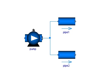
In such a case the balance equations define ideal mixing, i.e., the upstream discretization scheme of each component uses values that result from ideal mixing in an infinitely small time period. If more realistic modelling is desired that takes into account mixing losses, an explicit model has to be used in the connection point.
Single substance media
For a single substance medium, the connector definition in Modelica.Fluid.Interfaces.FluidPort reduces to
connector FluidPort
  replaceable package Medium = Modelica.Media.Interfaces.PartialMedium
    "Medium model of the fluid";
  flow Medium.MassFlowRate m_flow
    "Mass flow rate from the connection point into the component";
  Medium.AbsolutePressure p
    "Thermodynamic pressure in the connection point";
  stream Medium.SpecificEnthalpy h_outflow
    "Specific thermodynamic enthalpy close to the connection point if m_flow < 0";
end FluidPort;
The first statement defines the Medium flowing through the connector. In a medium, medium specific types such as "Medium.AbsolutePressure" are defined that contain medium specific values for the min, max and nominal attributes. Furthermore, Medium.MassFlowRate is defined as:
type MassFlowRate = SI.MassFlowRate(
  quantity = "MassFlowRate." + mediumName);
Generally, with the current library design, it is necessary to explicitly select the medium
model for each component in a circuit. This model is then propagated to the ports,
and a Modelica translator will check that the quantity and unit attributes
of connected interfaces are identical. Therefore, an error occurs,
if connected FluidPorts do not have a medium with the same medium name.
Automatic propagation of fluid models through the ports is not directly possible with the
Modelica 3.6 specification, but might be supported by the Modelica tool. For example,
in Dymola the option Advanced.MediaPropagation=1 can be set
to apply automatic propagation of media models in a circuit.
The thermodynamic pressure is an effort variable, which means that the connection of two or more ports states that the port pressures are the same.
The mass flow rate is a flow variable, which means that the connection of two or more ports states that the sum of all flow rates is zero.
The last variable is a stream variable, i.e., a specific quantity carried by the flow variable. The quantity on the connector always corresponds to the value close to the connection point, assuming that the fluid is flowing out of the connector, regardless of the actual direction of the flow. This helps avoiding singularities when the mass flow goes through zero. The stream properties for the other flow direction can be inquired with the built-in operator inStream(..), while the value of the stream variable corresponding to the actual flow direction can be inquired through the built-in operator actualStream(…).
The actual equations corresponding to these operators are introduced and solved automatically by the tool. In principle, they correspond to the balance equation sum(flow_variable) = 0 and sum(flow_variable*stream_variable_at_connection) = 0 applied to the set of connected ports. In this case the first equation is the mass balance sum(m_flow) = 0, and the second is the energy balance at the connection point sum(m_flow*h_connection) = 0.
In the simpler case of a one-to-one connections between port_a and port_b, inStream(port_a.h_outflow) just returns port_b.h_outflow. For multiple-way connections, mixing equations are generated, and special care is taken in order to avoid discontinuities around zero flow rates. For more details, see this presentation which illustrates the stream concept rationale and the underlying technicalities.
A connector should have only the minimal number of variables to describe the interface, otherwise there will be connection restrictions in certain cases. Therefore, in the connector no redundant variables are present, e.g., the temperature T is not present because it can be computed from the connector variables pressure p and specific enthalpy h.
Here are two simple examples to illustrate modeling with stream connectors. The first one is a rigid adiabatic volume mixing two flows, where the kinetic and gravitational terms in the energy balance are neglected for simplicity.
model MixingVolume "Volume that mixes two flows"
  import Modelica.Units.SI;
  replaceable package Medium = Modelica.Media.Interfaces.PartialPureSubstance;
  FluidPort port_a(redeclare package Medium = Medium) "Fluid connector a";
  FluidPort port_b(redeclare package Medium = Medium) "Fluid connector b";
  parameter SI.Volume V "Volume of device";
  SI.Mass             m "Mass in device";
  SI.Energy           U "Inner energy in device";
  Medium.BaseProperties medium(preferredMediumStates=true) "Medium in the device";
equation
  // Definition of port variables
  port_a.p         = medium.p;
  port_b.p         = medium.p;
  port_a.h_outflow = medium.h;  // The stream variable always corresponds to the
  port_b.h_outflow = medium.h;  // properties of the fluid holdup (outgoing flow)

  // Total quantities
  m = V*medium.d;
  U = m*medium.u;
  // Mass and energy balance (actualStream(..) is a built-in operator for streams to
  // compute the right h, depending on the flow direction)
  der(m) = port_a.m_flow + port_b.m_flow;
  der(U) = port_a.m_flow*actualStream(port_a.h_outflow) +
           port_b.m_flow*actualStream(port_b.h_outflow);
end MixingVolume;
The second example is the model of a component describing a lumped pressure loss between two ports, with no energy storage and no heat transfer. An isenthalpic transformation is assumed (changes in kinetic and potential energy between inlet and outlet are neglected).
model PressureLoss "Pressure loss component"
  replaceable package Medium = Modelica.Media.Interfaces.PartialPureSubstance;
  FluidPort port_a(redeclare package Medium = Medium) "Fluid connector a";
  FluidPort port_b(redeclare package Medium = Medium) "Fluid connector b";
  Medium.ThermodynamicState port_a_state_inflow "State at port_a if inflowing";
  Medium.ThermodynamicState port_b_state_inflow "State at port_b if inflowing";
  Medium.Density d_a "Density at port a if inflowing";
  Medium.Density d_b "Density at port b if inflowing";
  replaceable function f = SomeSpecificMassFlowFunction
    "Function to compute the mass flow rate";
equation
  // Medium states for inflowing fluid
  port_a_state_inflow = Medium.setState_phX(port_a.p, inStream(port_a.h_outflow));
  port_b_state_inflow = Medium.setState_phX(port_b.p, inStream(port_b.h_outflow));
  // Mass balance
  0 = port_a.m_flow + port_b.m_flow;
  // Instantaneous propagation of enthalpy flow between the ports with
  // isenthalpic state transformation (no storage and no loss of energy)
  port_a.h_outflow = inStream(port_b.h_outflow);
  port_b.h_outflow = inStream(port_a.h_outflow);
  // (Regularized) Momentum balance
  port_a.m_flow = f(port_a.p - port_b.p, d_a, d_b);
end PressureLoss;
If many such components are connected in series between two models with storage, the specific enthalpies are propagated in both directions and available to all pressure loss components, without problems when the mass flow goes through zero. The function f then uses either d_a or d_b depending on the sign of port_a.p-port_b.p, with a suitable regularization around zero to avoid discontinuities.
Please note that these models are highly idealized in order to explain the stream connector concept. Device models in the library are much more complete, handling issues such as initialization, steady vs. dynamic modelling, heat transfer from the outside, etc.
Multiple-substance media
Modelica.Fluid can handle models where the fluid contains multiple substances, so that its composition can be characterized by mass fraction vectors.
connector FluidPort
  replaceable package Medium = Modelica.Media.Interfaces.PartialMedium
    "Medium model of the fluid";
  flow Medium.MassFlowRate m_flow
    "Mass flow rate from the connection point into the component";
  Medium.AbsolutePressure p
    "Thermodynamic pressure in the connection point";
  stream Medium.SpecificEnthalpy h_outflow
    "Specific thermodynamic enthalpy close to the connection point if m_flow < 0";
  stream Medium.MassFraction Xi_outflow[Medium.nXi]
    "Independent mixture mass fractions m_i/m close to the connection point if m_flow < 0";
  stream Medium.ExtraProperty C_outflow[Medium.nC]
    "Properties c_i/m close to the connection point if m_flow < 0";
end FluidPort;
The mass fraction vectors Xi and C are also stream quantities, as they are carried by the mass flow rate. The corresponding connection equations are sum(m_flow*Xi) and sum(m_flow*C), which correspond to mass balances for the single substances. The vector Xi contains the mass fractions of the main components of the fluid, and is used together with p and h to determine the thermodynamic state of the fluid. The vector C contains the mass fraction of the trace components, which are accounted for in mass balances, but is ignored when computing the fluid properties. This allows to easily declare and use medium models with trace components starting from existing medium models (e.g., adding CO2 traces to Moist Air for air conditioning models).
Approximations in balance equations at connection point
Summing up, when two or more ports of the type FluidPort are connected, the following equations are generated by the tool:
sum(port_j.m_flow) = 0;               // Total Mass balance
port_j = port_k;                      // Momentum balance
sum(port_j.m_flow*h_connection) = 0;  // Energy balance
sum(port_j.m_flow*Xi_connection) = 0; // Single component mass balances
sum(port_j.m_flow*C_connection) = 0;  // Trace components mass balances
It is very important to bear in mind that
- the mass balances are always exact;
- the momentum and energy balance are only exact when two port with the same diameter are connected, because there is no friction and no change in fluid velocity.
In all other cases, i.e., different port diameters and/or multiple port connections:
- The momentum balance does not consider friction effects and changes of pressure due to changes in velocity.
- There might thus be errors in the momentum balance of the order of magnitude of the dynamic pressure ρv2/2.
- The energy balance does not consider the kinetic terms (gravity terms cancel out due to the infinitesimal size of the connection volume). There might thus be errors in the momentum balance of the order of magnitude of the kinetic energy v^2/2.
In many applications, where fluid speeds are low and thermal phenomena are mainly of interest, these approximations are commonly made and lead to acceptable results. In all other cases, explicit fitting and junction models should be used, that model explicitly all the kinetic phenomena with the appropriate level of detail.