WOLFRAM SYSTEM MODELER
WallFrictionWall friction |
|
Wolfram Language
In[1]:=
SystemModel["Modelica.Fluid.UsersGuide.ComponentDefinition.WallFriction"]
Out[1]:=
Information
This information is part of the Modelica Standard Library maintained by the Modelica Association.
One important special case for a pressure loss is the friction at the wall of a pipe under the assumption of quasi steady state flow (i.e., the mass flow rate varies only slowly). In this section it is explained how this case is handled in the Modelica.Fluid library for pipes with nonuniform roughness, including the smooth pipe as a special case (see Pipes.BaseClasses.WallFriction). The treatment is non-standard in order to get a numerically well-posed description.
For pipes with circular cross section the pressure drop is computed as:
   dp = λ(Re,Δ)*(L/D)*ρ*v*|v|/2
      = λ(Re,Δ)*8*L/(π^2*D^5*ρ)*m_flow*|m_flow|
      = λ2(Re,Δ)*k2*sign(m_flow);

with
   Re     = |v|*D*ρ/μ
          = |m_flow|*4/(π*D*μ)
   m_flow = A*v*ρ
   A      = π*(D/2)^2
   λ2     = λ*Re^2
   k2     = L*μ^2/(2*D^3*ρ)
where
- L is the length of the pipe.
- D is the diameter of the pipe. If the pipe has not a circular cross section, D = 4*A/P, where A is the cross section area and P is the wetted perimeter.
- λ = λ(Re,Δ) is the "usual" wall friction coefficient.
- λ2 = λ*Re^2 is the used friction coefficient to get a numerically well-posed formulation.
- Re = |v|*D*ρ/μ is the Reynolds number.
- Δ = δ/D is the relative roughness where "δ" is the absolute "roughness", i.e., the averaged height of asperities in the pipe (δ may change over time due to growth of surface asperities during service, see [Idelchik 1994, p. 85, Tables 2-1, 2-2]).
- ρ is the upstream density.
- μ is the upstream dynamic viscosity.
- v is the mean velocity.
The first form with λ is used and presented in textbooks, see "blue" curve in the next figure:
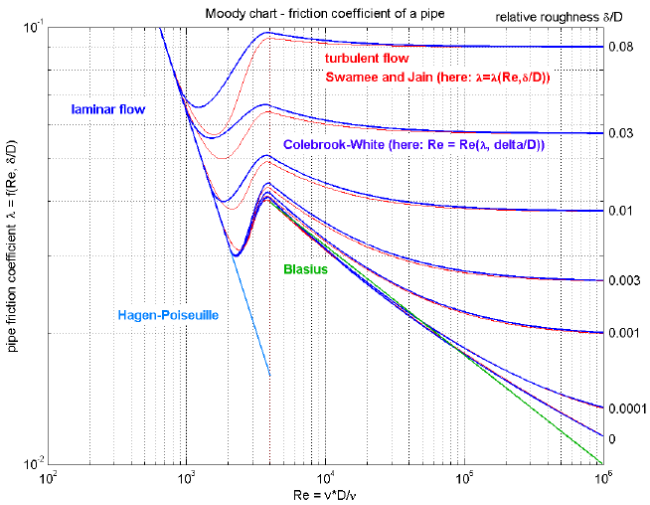
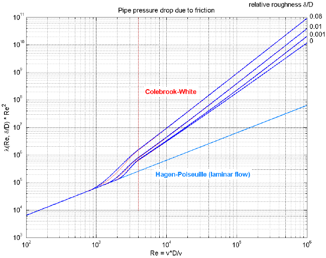
This form is not suited for a simulation program since λ = 64/Re if Re < 2000, i.e., a division by zero occurs for zero mass flow rate because Re = 0 in this case. More useful for a simulation model is the friction coefficient λ2 = λ*Re^2, because λ2 = 64*Re if Re < 2000 and therefore no problems for zero mass flow rate occur. The characteristic of λ2 is shown in the next figure and is used in Modelica.Fluid:
The pressure loss characteristic is divided into three regions:
- Region 1:
For Re ≤ 2000, the flow is laminar and the exact solution of the
3-dim. Navier-Stokes equations (momentum and mass balance) is used under the
assumptions of steady flow, constant pressure gradient and constant
density and viscosity (= Hagen-Poiseuille flow) leading to λ2 = 64*Re.
Therefore:
dp = 128*μ*L/(π*D^4*ρ)*m_flow - Region 3:
For Re ≥ 4000, the flow is turbulent.
Depending on the calculation direction (see "inverse formulation"
below) either of two explicit equations are used. If the pressure drop dp
is assumed to be known, λ2 = |dp|/k2. The
Colebrook-White equation
[Colebrook 1939; Idelchik 1994, p. 83, eq. (2-9)]:
gives an implicit relationship between Re and λ. Inserting λ2 = λ*Re^2 allows to solve this equation analytically for Re:1/sqrt(λ) = -2*lg( 2.51/(Re*sqrt(λ)) + 0.27*Δ)
Finally, the mass flow rate m_flow is computed from Re via m_flow = Re*π*D*μ/4*sign(dp). These are the red curves in the diagrams above.Re = -2*sqrt(λ2)*lg(2.51/sqrt(λ2) + 0.27*Δ)
If the mass flow rate is assumed known (and therefore implicitly also the Reynolds number), then λ2 is computed by an approximation of the inverse of the Colebrook-White equation [Swamee and Jain 1976; Miller 1990, p. 191, eq.(8.4)] adapted to λ2:
The pressure drop is then computed as dp = k2*λ2*sign(m_flow). These are the blue curves in the diagrams above.λ2 = 0.25*(Re/lg(Δ/3.7 + 5.74/Re^0.9))^2
- Region 2:
For 2000 ≤ Re ≤ 4000 there is a transition region between laminar
and turbulent flow. The value of λ2 depends on more factors as just
the Reynolds number and the relative roughness, therefore only crude
approximations are possible in this area.
The deviation from the laminar region depends on the relative roughness. A laminar flow at Re=2000 is only reached for smooth pipes. The deviation Reynolds number Re1 is computed according to [Samoilenko 1968; Idelchik 1994, p. 81, sect. 2.1.21] as:
These are the blue curves in the diagrams above.Re1 = 745*e^(if Δ ≤ 0.0065 then 1 else 0.0065/Δ)
Between Re1=Re1(δ/D) and Re2=4000, λ2 is approximated by a cubic polynomial in the "lg(λ2) - lg(Re)" chart (see figures above) such that the first derivative is continuous at these two points. In order to avoid the solution of non-linear equations, two different cubic polynomials are used for the direct and the inverse formulation. This leads to some discrepancies in λ2 (= differences between the red and the blue curves). This is acceptable, because the transition region is anyway not precisely known since the actual friction coefficient depends on additional factors and since the operating points are usually not in this region.
The absolute roughness δ has usually to be estimated. In [Idelchik 1994, pp. 105-109, Table 2-5; Miller 1990, p. 190, Table 8-1] many examples are given. As a short summary:
| Smooth pipes | Drawn brass, copper, aluminium, glass, etc. | δ = 0.0025 mm |
| Steel pipes | New smooth pipes | δ = 0.025 mm |
| Mortar lined, average finish | δ = 0.1 mm | |
| Heavy rust | δ = 1 mm | |
| Concrete pipes | Steel forms, first class workmanship | δ = 0.025 mm |
| Steel forms, average workmanship | δ = 0.1 mm | |
| Block linings | δ = 1 mm |
The equations above are valid for incompressible flow. They can also be applied for compressible flow up to about Ma = 0.6 (Ma is the Mach number) with a maximum error in λ of about 3 %. The effect of gas compressibility in a wide region can be taken into account by the following formula derived by Voronin [Voronin 1959; Idelchik 1994, p. 97, sect. 2.1.81]:
λ_comp = λ*(1 + (κ-1)/2 * Ma^2)^(-0.47)
where κ is the isentropic coefficient (for ideal gases, κ is the ratio of specific heat capacities cp/cv). An appreciable decrease in the coefficient "λ_comp" is observed only in a narrow transonic region and also at supersonic flow velocities by about 15% [Idelchik 1994, p. 97, sect. 2.1.81]. This effect is not yet included in Modelica.Fluid. Another restriction is that the pressure drop model is valid only for steady state or slowly changing mass flow rate. For large fluid acceleration, the pressure drop depends additionally on the frequency of the changing mass flow rate.
Inverse formulation
In the "Advanced menu" it is possible via parameter "from_dp" to define in which form the pressure drop equation is actually evaluated (default is from_dp = true):
from_dp = true:   m_flow = f1(dp)
        = false:  dp     = f2(m_flow)
"from_dp" can be useful to avoid nonlinear systems of equations in cases where the inverse pressure loss function is needed.
Summary
A detailed pressure drop model for pipe wall friction is provided in the form m_flow = f1(dp, Δ) or dp = f2(m_flow, Δ). These functions are continuous and differentiable, are provided in an explicit form without solving non-linear equations, and do behave well also at small mass flow rates. This pressure drop model can be used stand-alone in a static momentum balance and in a dynamic momentum balance as the friction pressure drop term. It is valid for incompressible and compressible flow up to a Mach number of 0.6.
References
- Colebrook F. (1939):
- Turbulent flow in pipes with particular reference to the transition region between the smooth and rough pipe laws. J. Inst. Civ. Eng. no. 4, 14-25.
- Idelchik I.E. (1994):
- Handbook of Hydraulic Resistance. 3rd edition, Begell House, ISBN 0-8493-9908-4
- Miller D. S. (1990):
- Internal flow systems. 2nd edition. Cranfield:BHRA(Information Services).
- Samoilenko L.A. (1968):
- Investigation of the Hydraulic Resistance of Pipelines in the Zone of Transition from Laminar into Turbulent Motion. Thesis (Cand. of Technical Science), Leningrad.
- Swamee P.K. and Jain A.K. (1976):
- Explicit equations for pipe-flow problems. Proc. ASCE, J.Hydraul. Div., 102 (HY5), pp. 657-664.
- Voronin F.S. (1959):
- Effect of contraction on the friction coefficient in a turbulent gas flow. Inzh. Fiz. Zh., vol. 2, no. 11, pp. 81-85.