2.4.3 Circuit Equation Formulations

Modified Nodal Analysis

The modified nodal analysis method (MNA) has already been introduced as the default formulation by which Analog Insydes sets up circuit equations. The MNA formulation is general, yields relatively compact systems of equations, and is easy to implement on a computer. These and a few other favorable properties have made it the most widely used analysis method in electrical circuit simulators, including Analog Insydes.

There are a number of user-settable options which have an influence on the way Analog Insydes sets up MNA equations. You have already encountered the netlist option Pattern which specifies explicitly whether to use the impedance or admittance fill-in pattern for an immittance element, i.e. a two-terminal admittance or impedance. This option allows, for instance, to prevent the implicit conversion of an impedance to an admittance, thereby augmenting the MNA system by the branch current of the impedance. However, the Pattern option pertains only to the element in whose value field it is given. To prevent implicit impedance conversion globally you can set the value of the CircuitEquations option ConvertImmittances to False, either permanently by modifying Options[CircuitEquations] using the SetOptions directive, or temporarily by passing the option ConvertImmittances -> False to the function CircuitEquations:

In[8]:= CircuitEquations[rlcfilter,
ConvertImmittances -> False] // DisplayForm

Out[8]//DisplayForm=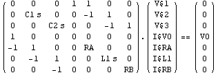

The Formulation Option

With modified nodal analysis being the default analysis method there is usually no need to request this formulation explicitly. However, if you have changed the default settings in Options[CircuitEquations] or if you wish to use one of the analysis methods to be discussed in the following subsections you need to specify the formulation as an option to CircuitEquations. The option keyword is Formulation, and the option value can be either ModifiedNodal, SparseTableau, or ExtendedTableau. Hence, modified nodal analysis can be explicitly selected by this command:

In[9]:= CircuitEquations[rlcfilter,
Formulation -> ModifiedNodal] // DisplayForm

Out[9]//DisplayForm=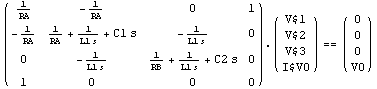

Sparse Tableau Analysis: The Basic Formulation

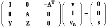
In addition to nodal analysis, Analog Insydes also offers the possibility to set up circuit equations according to two variants of the sparse tableau formulation (STA). For an electrical network containing electrical branches, the basic variant of the sparse tableau comprises the topological node and loop equations resulting from Kirchhoff's voltage law (KVL) and current law (KCL), plus the voltage-current relations of the circuit elements. Hence, the basic sparse tableau forms the following matrix equation in terms of the branch voltages v and the branch currents i.

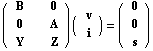
Here, A denotes the nodal incidence matrix of the network graph and B a loop incidence matrix of maximum rank. B is derived automatically from A by an algorithm which searches for a tree in the network graph and then extracts the fundamental loop matrix defined by that tree. The matrices Y and Z in the third row of the tableau represent the coefficient matrices of the element relations. On the right-hand side, s denotes the contribution of the independent sources. All remaining tableau entries are structurally zero (0).

In[10]:= CircuitEquations[rlcfilter,
Formulation -> SparseTableau] // DisplayForm

Out[10]//DisplayForm=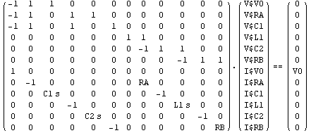

Sparse Tableau Analysis: The Extended Formulation

Analog Insydes also supports an extended sparse tableau formulation in which the vector of unknowns comprises the branch voltages v, the branch currents i, and the node voltages . With I denoting an identity matrix of rank and the transpose of the nodal incidence matrix A, Kirchhoff's voltage law is expressed indirectly in terms of the node voltages as . Therefore, the extended sparse tableau formulation does not require the calculation of a loop matrix, though at the expense of a larger matrix size than that of the basic variant:

The extended variant is selected by the option setting Formulation -> ExtendedTableau:

In[11]:= rlcstaext = CircuitEquations[rlcfilter,
Formulation -> ExtendedTableau];
DisplayForm[rlcstaext]

Out[12]//DisplayForm=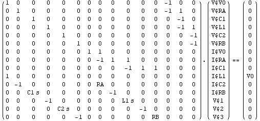

Of course, the solution for a particular quantity in a circuit does not depend on the type of equations from which the solution is computed. So the value for V$3 obtained by an extended sparse tableau analysis is identical to the one computed by modified nodal analysis:

In[12]:= V$3 /. First[Solve[rlcstaext, V$3]]

Out[13]=