|
2.4.4 Additional Options for CircuitEquations
All Analog Insydes options which have an influence on circuit equation setup by the function CircuitEquations can be accessed through Options[CircuitEquations]. The current option settings can be inspected by retrieving the value of this variable:
In[13]:= Options[CircuitEquations]
Out[14]= 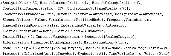
Some of these options are discussed in more detail below.
AnalysisMode
CircuitEquations sets up circuit equations for the analysis modes AC, DC, and transient. Which mode to use is determined by the option AnalysisMode, whose value is one of the symbols AC, DC, and Transient. The default value is AC. Up to now, we used CircuitEquations to create small-signal equations. Section 2.6.4 describes how to set up DC equations and Section 2.7.1 describes how to set up transient equations.
MatrixEquation
Using the option MatrixEquation -> False, we can force CircuitEquations not to use a matrix representation when setting up small-signal circuit equations but to return a list of scalar equations instead.
In[14]:= CircuitEquations[rlcfilter,
MatrixEquation -> False] // DisplayForm
Out[15]//DisplayForm= 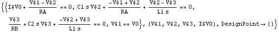
When the matrix representation is turned off, the value returned by CircuitEquations is a DAEObject containing the circuit equations as a list of two elements, the first being the system of circuit equations and the second the vector of unknowns. The advantage of the scalar representation is that it consumes less memory than the matrix representation because Mathematica does not have a special storage mechanism for sparse matrices. Nevertheless, some commands (e.g. ACAnalysis) rely on the fact that the equation system is formulated in matrix representation.
FrequencyVariable
The option FrequencyVariable -> symbol specifies the symbol which Analog Insydes uses to denote the differential operator, i.e. the complex frequency, in the Laplace domain. By default, this is the symbol s, but if you prefer to use another symbol for this purpose, for instance p, you can replace s by p as follows:
In[15]:= CircuitEquations[rlcfilter,
FrequencyVariable -> p] // DisplayForm
Out[16]//DisplayForm= 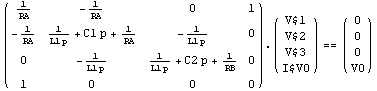
ElementValues
With ElementValues -> Symbolic we can instruct CircuitEquations to use the symbolic values from the value fields of netlist entries in which a Symbolic option is given. To demonstrate the effect of this option let's make some enhancements to the netlist of the RLC filter circuit from Section 2.4.2 (see Figure 4.1). Using the extended value-field format (see Section 3.1.4) we specify a numerical as well as a symbolic value for the circuit elements.
In[16]:= rlcfilter2 =
Netlist[
{V0, {1, 0}, Value -> V0, Symbolic -> V0},
{RA, {1, 2}, Value -> 1000., Symbolic -> RA},
{C1, {2, 0}, Value -> 4.7*10^-6, Symbolic -> C1},
{L1, {2, 3}, Value -> 1.0*10^-3, Symbolic -> L1},
{C2, {3, 0}, Value -> 2.2*10^-5, Symbolic -> C2},
{RB, {3, 0}, Value -> 1000., Symbolic -> RB}
];
Note that the value of the Symbolic option needs not to coincide with the reference designator as this is the case in the example above. You can use any Mathematica expression as value to the Symbolic field.
A call to CircuitEquations without any additional options (i.e. the default value of the ElementValues option is used, which is Value) will then cause the numerical values to be entered into the matrix as these are given as arguments to the Value rules.
In[17]:= rlc2eqs = CircuitEquations[rlcfilter2];
DisplayForm[rlc2eqs]
Out[19]//DisplayForm= 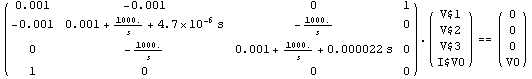
Alternatively, we can select the symbolic values by means of the option ElementValues -> Symbolic. Note that ElementValues affects only those netlist entries in whose value field a Symbolic rule is present.
In[18]:= rlc2eqs2 = CircuitEquations[rlcfilter2,
ElementValues -> Symbolic];
DisplayForm[rlc2eqs2]
Out[21]//DisplayForm= 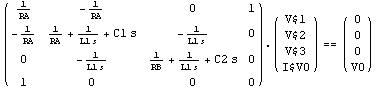
|