LeastSquares
LeastSquares[m,b]
finds an x that solves the linear least-squares problem for the matrix equation m.x==b.
Details and Options
- LeastSquares[m,b] gives a vector x that minimizes Norm[m.x-b].
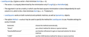
- The vector x is uniquely determined by the minimization only if Length[x]==MatrixRank[m].
- The argument b can be a matrix, in which case the least-squares minimization is done independently for each column in b, which is the x that minimizes Norm[m.x-b,"Frobenius"].
- LeastSquares works on both numerical and symbolic matrices, as well as SparseArray objects.
- The option Methodmethod may be used to specify the method for LeastSquares to use. Possible settings for method include:
-
Automatic choose the method automatically "Direct" use a direct method for dense or sparse matrices "IterativeRefinement" use iterative refinement to get an improved solution for dense matrices "LSQR" use the LSQR iterative method for dense or sparse machine number matrices "Krylov" use an iterative method for sparse machine number matrices
Examples
open allclose allBasic Examples (2)
Solve a simple least-squares problem:
This finds a tuple ![]() that minimizes
that minimizes ![]() :
:
Use LeastSquares to minimize ![]() :
:
Compare to general minimization:
Note there is no solution to ![]() , so
, so ![]() may be regarded as the best approximate solution:
may be regarded as the best approximate solution:
Scope (11)
Basic Uses (7)
Find the least squares for a machine-precision matrix:
Least squares for a complex matrix:
Use LeastSquares for an exact non-square matrix:
Least squares for an arbitrary-precision matrix:
Use LeastSquares with a symbolic matrix:
The least squares for a large numerical matrix is computed efficiently:
In LeastSquares[m,b], b can be a matrix:
Each column in the result equals the solution found by using the corresponding column in b as input:
Special Matrices (4)
Solve a least-squares problem for a sparse matrix:
Solve the least-squares problem with structured matrices:
Use a different type of matrix structure:
LeastSquares[IdentityMatrix[n],b] gives the vector ![]() :
:
Least squares of HilbertMatrix:
Options (1)
Tolerance (1)
m is a 20×20 Hilbert matrix, and b is a vector such that the solution of m.x==b is known:
With the default tolerance, numerical roundoff is limited, so errors are distributed:
With Tolerance->0, numerical roundoff can introduce excessive error:
Specifying a higher tolerance will limit roundoff errors at the expense of a larger residual:
Applications (9)
Geometry of Least Squares (4)
LeastSquares[m,b] can be understood as finding the solution to ![]() , where
, where ![]() is the orthogonal projection of
is the orthogonal projection of ![]() onto the column space of
onto the column space of ![]() . Consider the following
. Consider the following ![]() and
and ![]() :
:
Find an orthonormal basis for the space spanned by the columns of ![]() :
:
Compute the orthogonal projection![]() of
of ![]() onto the spaced spanned by the
onto the spaced spanned by the ![]() :
:
Visualize ![]() , its projections
, its projections ![]() onto the
onto the ![]() , and
, and ![]() :
:
This is the same result as given by LeastSquares:
Compare and explain the answers returned by LeastSquares[m,b] and LinearSolve[m,b⟂] for the following ![]() and
and ![]() :
:
Find an orthonormal basis for the space spanned by the columns of ![]() :
:
A zero vector is returned because the rank of the matrix is less than the number of columns:
Compute the orthogonal projection![]() of
of ![]() onto the spaced spanned by the
onto the spaced spanned by the ![]() :
:
Find the solution returned by LeastSquares:
While x and xPerp are different, both solve the least-squares problem because m.x==m.xPerp:
The two solutions differ by an element of NullSpace[m]:
Use the matrix projection operators for a matrix with linearly independent columns to find LeastSquares[m,b] for the following ![]() and
and ![]() :
:
The projection operator on the column space of ![]() is
is ![]() :
:
The solution to the least-squares problem is then the unique solution to ![]() :
:
Confirm using LeastSquares:
Compare the solutions found using LeastSquares[m,b] and LinearSolve together with the normal equations of ![]() and for the following
and for the following ![]() and
and ![]() :
:
Solve using LeastSquares:
Solve using LinearSolve and the normal equations ![]() :
:
While x and xNormal are different, both solve the least-squares problem because m.x==m.xNormal:
The two solutions differ by an element of NullSpace[m]:
Curve and Parameter Fitting (5)
LeastSquares can be used to find a best-fit curve to data. Consider the following data:
Extract the ![]() and
and ![]() coordinates from the data:
coordinates from the data:
Let ![]() have the columns
have the columns ![]() and
and ![]() , so that minimizing
, so that minimizing ![]() will be fitting to a line
will be fitting to a line ![]() :
:
Get the coefficients ![]() and
and ![]() for a linear least‐squares fit:
for a linear least‐squares fit:
Verify the coefficients using Fit:
Plot the best-fit curve along with the data:
Find the best-fit parabola to the following data:
Extract the ![]() and
and ![]() coordinates from the data:
coordinates from the data:
Let ![]() have the columns
have the columns ![]() ,
, ![]() and
and ![]() , so that minimizing
, so that minimizing ![]() will be fitting to
will be fitting to ![]() :
:
Get the coefficients ![]() ,
, ![]() and
and ![]() for a least‐squares fit:
for a least‐squares fit:
Verify the coefficients using Fit:
Plot the best-fit curve along with the data:
A healthy child’s systolic blood pressure ![]() (in millimeters of mercury) and weight
(in millimeters of mercury) and weight ![]() (in pounds) are approximately related by the equation
(in pounds) are approximately related by the equation ![]() . Use the following experimental data points
. Use the following experimental data points ![]() to estimate the systolic blood pressure of a healthy child weighing 100 pounds:
to estimate the systolic blood pressure of a healthy child weighing 100 pounds:
Use DesignMatrix to construct the matrix with columns ![]() and
and ![]() :
:
Extract the ![]() values from the data:
values from the data:
The least-squares solution of ![]() :
:
Substitute the parameters into the model:
Then the expected blood pressure of a child weighing 100 pounds is roughly ![]() :
:
Visualize the best-fit curve and the data:
According to Kepler’s first law, a comet's orbit satisfies ![]() , where
, where ![]() is a constant and
is a constant and ![]() is the eccentricity. The eccentricity determines the type of orbit, with
is the eccentricity. The eccentricity determines the type of orbit, with ![]() for an ellipse,
for an ellipse, ![]() for a parabola, and
for a parabola, and ![]() for a hyperbola. Use the following observational data to determine the type of orbit of the comet and predict its distance from the Sun at
for a hyperbola. Use the following observational data to determine the type of orbit of the comet and predict its distance from the Sun at ![]() :
:
To find ![]() and
and ![]() , first use DesignMatrix to create the matrix whose columns are
, first use DesignMatrix to create the matrix whose columns are ![]() and
and ![]() :
:
Use LeastSquares to find the ![]() and
and ![]() that minimize the error in
that minimize the error in ![]() from the design matrix:
from the design matrix:
Since ![]() , the orbit is elliptical and there is a unique value of
, the orbit is elliptical and there is a unique value of ![]() for each value of
for each value of ![]() :
:
Evaluating the function at ![]() gives an expected distance of roughly
gives an expected distance of roughly ![]() :
:
Extract the ![]() and
and ![]() coordinates from the data:
coordinates from the data:
Define cubic basis functions centered at t with support on the interval [t-2,t+2]:
Set up a sparse design matrix for basis functions centered at 0, 1, ..., 10:
Solve the least-squares problem:
Visualize the data with the best-fit piecewise cubic, which is ![]() :
:
Properties & Relations (12)
If m.x==b can be solved, LeastSquares is equivalent to LinearSolve:
If x=LeastSquares[m,b] and n lies in NullSpace[m], x+n is also a least-squares solution:
LeastSquares[m,b] solves ![]() , with
, with ![]() the orthogonal projection onto the columns of
the orthogonal projection onto the columns of ![]() :
:
Equality was guaranteed because this particular matrix has a trivial null space:
If ![]() is real valued, x=LeastSquares[m,b] obeys the normal equations
is real valued, x=LeastSquares[m,b] obeys the normal equations ![]() :
:
For a complex-valued matrix, the equations are ![]() :
:
Given x==LeastSquares[m,b], m.x-b lies in NullSpace[ConjugateTranspose[m]]:
The null space is two dimensional:
m.ls-b lies in the span for the two vectors, as expected:
LeastSquares and PseudoInverse can both be used to solve the least-squares problem:
LeastSquares and QRDecomposition can both be used to solve the least-squares problem:
Let m be a matrix with an empty nullspace:
For a vector b, LeastSquares[m,b] is equivalent to ArgMin[Norm[m.x-b],x]:
It is also equivalent to ArgMin[Norm[m.x-b,"Frobenius"],x]:
Let m be a matrix with an empty nullspace:
For a matrix b, LeastSquares is equivalent to ArgMin[Norm[m.x-b,"Frobenius"],x]:
If b is a matrix, each column in LeastSquares[m,b] is the result for the corresponding column in b:
m is a 5×2 matrix, and b is a length-5 vector:
Solve the least-squares problem:
It is also gives the coefficients for the line with least-squares distance to the points:
LeastSquares gives the parameter estimates for a linear model with normal errors:
LinearModelFit fits the model and gives additional information about the fitting:
Text
Wolfram Research (2007), LeastSquares, Wolfram Language function, https://reference.wolfram.com/language/ref/LeastSquares.html (updated 2021).
CMS
Wolfram Language. 2007. "LeastSquares." Wolfram Language & System Documentation Center. Wolfram Research. Last Modified 2021. https://reference.wolfram.com/language/ref/LeastSquares.html.
APA
Wolfram Language. (2007). LeastSquares. Wolfram Language & System Documentation Center. Retrieved from https://reference.wolfram.com/language/ref/LeastSquares.html