TimeSeriesForecast
TimeSeriesForecast[tproc,data,k]
gives the k-step-ahead forecast beyond data according to the time series process tproc.
TimeSeriesForecast[tsmod,k]
gives the k-step-ahead forecast for TimeSeriesModel tsmod.
Details and Options
- TimeSeriesForecast[tproc,{x0,…,xm},k] will give Expectation[x[m+k]x[0]x0∧…∧x[m]xm], where xtproc, the expected value of the process given data.
- TimeSeriesForecast allows tproc to be a time series process such as ARProcess, ARMAProcess, SARIMAProcess, etc.
- The data can be a list of numeric values {x1,x2,…}, a list of time-value pairs {{t1,x1},{t2,x2},…}, or TemporalData.
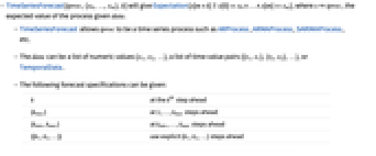
- The following forecast specifications can be given:
-
k at the k ") step ahead
step ahead{kmax} at 1, …, kmax steps ahead {kmin,kmax} at kmin, …, kmax steps ahead {{k1,k2,…}} use explicit {k1,k2,…} steps ahead - TimeSeriesForecast returns the forecasted value if k is an integer and TemporalData otherwise.
- The default for k is 1.
- TimeSeriesForecast supports a Method option with the following settings:
-
Automatic automatically determine the method "AR" approximate with a large-order AR process "Covariance" exact covariance function-based "Kalman" use Kalman filter - The mean squared errors of the prediction are the compounded noise errors and are given as MetaInformation in the TemporalData output. For forecast=TimeSeriesForecast[tproc,data,k], the mean squared errors can be accessed by forecast["MeanSquaredErrors"].
Examples
open allclose allBasic Examples (3)
Forecast three steps ahead for an ARProcess:
An ARMAProcess:
Predict the seventh value from TimeSeriesModel:
Mean squared error of the forecast:
Forecast a vector-valued time series process:
Scope (7)
Step (4)
Mean Squared Errors (3)
Return the forecast as TemporalData to extract mean squared errors:
Find the forecast with mean squared errors:
Plot the data and forecast with mean error bands:
Find the forecast with 95% confidence intervals:
Find the forecast for the next 10 steps:
Options (4)
Method (4)
Find the forecast using the covariance-based method:
Find the forecast using the autoregressive method:
Find the forecast using the Kalman filter method:
Compare exact and approximate methods for an MAProcess:
Applications (3)
The daily exchange rates of the euro to the dollar from May 2012 through September 2012:
Fit an AR process to the exchange rates:
Forecast for 20 business days ahead:
Plot the forecast with original data:
Consider hourly temperature readings for September 9, 2012, near your location:
The data contains missing values:
Redefine time series with MissingDataMethod to fill in missing data with interpolated values:
Check if the time stamps are regularly spaced:
Estimate an ARProcess:
Calculate prediction for the next 12 hours:
Plot forecast with original data:
Retail monthly sales in United States:
Create TimeSeries from the selection:
Plot the sales with grid lines at December peaks:
Find forecast for the next 7 years:
Calculate 95% confidence bands for the forecast:
Properties & Relations (3)
Forecasting with ARProcess using the exact or approximate method gives the same result:
Forecast is the same for a time series process and its invertible representation:
This process is not invertible:
Find its invertible representation:
Use TimeSeriesModel to forecast:
Compute forecast for 20 steps:
Text
Wolfram Research (2012), TimeSeriesForecast, Wolfram Language function, https://reference.wolfram.com/language/ref/TimeSeriesForecast.html (updated 2014).
CMS
Wolfram Language. 2012. "TimeSeriesForecast." Wolfram Language & System Documentation Center. Wolfram Research. Last Modified 2014. https://reference.wolfram.com/language/ref/TimeSeriesForecast.html.
APA
Wolfram Language. (2012). TimeSeriesForecast. Wolfram Language & System Documentation Center. Retrieved from https://reference.wolfram.com/language/ref/TimeSeriesForecast.html