"ExplicitRungeKutta" Method for NDSolve
| Introduction | Stiffness |
| Example | Stiffness Detection |
| Method Comparison | Step Control Revisited |
| Coefficient Plug-in | Option Summary |
| Method Plug-in |
Introduction
Euler's Method
One of the first and simplest methods for solving initial value problems was proposed by Euler:
Euler's method is not very accurate.
Local accuracy is measured by how high terms are matched with the Taylor expansion of the solution. Euler's method is first-order accurate, so that errors occur one order higher starting at powers of ![]() .
.
Generalizing Euler's Method
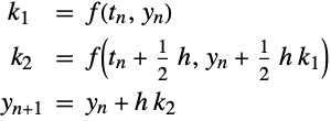
The idea of Runge–Kutta methods is to take successive (weighted) Euler steps to approximate a Taylor series. In this way function evaluations (and not derivatives) are used.
The midpoint method can be shown to have a local error of ![]() , so it is second-order accurate.
, so it is second-order accurate.
Runge–Kutta Methods
Extending the approach in (1), repeated function evaluation can be used to obtain higher-order methods.
Denote the Runge–Kutta method for the approximate solution to an initial value problem at ![]() by
by
where ![]() is the number of stages.
is the number of stages.
It is generally assumed that the row-sum conditions hold:
These conditions effectively determine the points in time at which the function is sampled and are a particularly useful device in the derivation of high-order Runge–Kutta methods.
The coefficients of the method are free parameters that are chosen to satisfy a Taylor series expansion through some order in the time step ![]() . In practice other conditions such as stability can also constrain the coefficients.
. In practice other conditions such as stability can also constrain the coefficients.
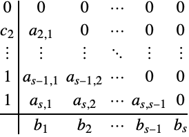
Explicit Runge–Kutta methods are a special case where the matrix ![]() is strictly lower triangular:
is strictly lower triangular:
It has become customary to denote the method coefficients ![]() ,
, ![]() , and
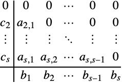
, and ![]() using a Butcher table, which has the following form for explicit Runge–Kutta methods.
using a Butcher table, which has the following form for explicit Runge–Kutta methods.
The row-sum conditions can be visualized as summing across the rows of the table.
Notice that a consequence of explicitness is ![]() , so that the function is sampled at the beginning of the current integration step.
, so that the function is sampled at the beginning of the current integration step.
Example
The Butcher table for the explicit midpoint method (2) is given by:
FSAL Schemes
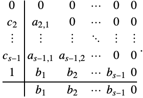
A particularly interesting special class of explicit Runge–Kutta methods, used in most modern codes, is that for which the coefficients have a special structure known as First Same As Last (FSAL):
For consistent FSAL schemes the Butcher table (3) has the form:
The advantage of FSAL methods is that the function value ![]() at the end of one integration step is the same as the first function value
at the end of one integration step is the same as the first function value ![]() at the next integration step.
at the next integration step.
The function values at the beginning and end of each integration step are required anyway when constructing the InterpolatingFunction that is used for dense output in NDSolve.
Embedded Pairs and Local Error Estimation
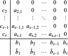
An efficient means of obtaining local error estimates for adaptive step-size control is to consider two methods of different orders ![]() and
and ![]() that share the same coefficient matrix (and hence function values).
that share the same coefficient matrix (and hence function values).
A commonly used notation is ![]() , typically with
, typically with ![]() or
or ![]() .
.
In most modern codes, including the default choice in NDSolve, the solution is advanced with the more accurate formula so that ![]() , which is known as local extrapolation.
, which is known as local extrapolation.
The vector of coefficients ![]() gives an error estimator avoiding subtractive cancellation of
gives an error estimator avoiding subtractive cancellation of ![]() in floating-point arithmetic when forming the difference between (4) and (5).
in floating-point arithmetic when forming the difference between (4) and (5).
The quantity ![]() gives a scalar measure of the error that can be used for step size selection.
gives a scalar measure of the error that can be used for step size selection.
Step Control
The classical Integral (or I) step-size controller uses the formula
The error estimate is therefore used to determine the next step size to use from the current step size.
The notation ![]() is explained within "Norms in NDSolve".
is explained within "Norms in NDSolve".
Overview
Explicit Runge–Kutta pairs of orders 2(1) through 9(8) have been implemented.
Formula pairs have the following properties:
- Stiffness detection capability (see "StiffnessTest Method Option for NDSolve").
- Proportional-Integral step-size controller for stiff and quasi-stiff systems [G91].
Optimal formula pairs of orders 2(1), 3(2), and 4(3) subject to the already stated requirements have been derived using the Wolfram Language, and are described in [SS04].
The 5(4) pair selected is due to Bogacki and Shampine [BS89b, S94] and the 6(5), 7(6), 8(7), and 9(8) pairs are due to Verner [V10].
For the selection of higher-order pairs, issues such as local truncation error ratio and stability region compatibility should be considered (see [S94]). Various tools have been written to assess these qualitative features.
Methods are interchangeable so that, for example, it is possible to substitute the 5(4) method of Bogacki and Shampine with a method of Dormand and Prince.
Summation of the method stages is implemented using level 2 BLAS which is often highly optimized for particular processors and can also take advantage of multiple cores.
Example
Method Comparison
Sometimes you may be interested to find out what methods are being used in NDSolve.
You also may want to compare some of the different methods to see how they perform for a specific problem.
Utilities
You will make use of a utility function CompareMethods for comparing various methods. Some useful NDSolve features of this function for comparing methods are:
- The option EvaluationMonitor, which is used to count the number of function evaluations.
- The option StepMonitor, which is used to count the number of accepted and rejected integration steps.
Reference Solution
A number of examples for comparing numerical methods in the literature rely on the fact that a closed-form solution is available, which is obviously quite limiting.
In NDSolve it is possible to get very accurate approximations using arbitrary-precision adaptive step size; these are adaptive order methods based on "Extrapolation".
Automatic Order Selection
When you select "DifferenceOrder"->Automatic, the code will automatically attempt to choose the optimal order method for the integration.
Two algorithms have been implemented for this purpose and are described within "SymplecticPartitionedRungeKutta Method for NDSolve".
Example 1
Here is an example that compares built-in methods of various orders, together with the method that is selected automatically.
The default method has order nine, which is close to the optimal order of eight in this example. One function evaluation is needed during the initialization phase to determine the order.
Example 2
A limitation of the previous example is that it did not take into account the accuracy of the solution obtained by each method, so that it did not give a fair reflection of the cost.
Rather than taking a single tolerance to compare methods, it is preferable to use a range of tolerances.
The following example compares various "ExplicitRungeKutta" methods of different orders using a variety of tolerances.
The order-selection algorithms are heuristic in that the optimal order may change through the integration but, as the examples illustrate, a reasonable default choice is usually made.
Ideally, a selection of different problems should be used for benchmarking.
Coefficient Plug-in
The implementation of "ExplicitRungeKutta" provides a default method pair at each order.
Sometimes, however, it is convenient to use a different method, for example:
The Classical Runge–Kutta Method
The method has no embedded error estimate and hence there is no specification of the coefficient error vector. This means that the method is invoked with fixed step sizes.
ode23
This defines the coefficients for a 3(2) FSAL explicit Runge–Kutta pair.
The third-order formula is due to Ralston, and the embedded method was derived by Bogacki and Shampine [BS89a].
The method is used in the Texas Instruments TI-85 pocket calculator, Matlab, and RKSUITE [S94]. Unfortunately it does not allow for the form of stiffness detection that has been chosen.
A Method of Fehlberg
This defines the coefficients for a 4(5) explicit Runge–Kutta pair of Fehlberg that was popular in the 1960s [F69].
The fourth-order formula is used to propagate the solution, and the fifth-order formula is used only for the purpose of error estimation.
In contrast to the classical Runge–Kutta method of order four, the coefficients include an additional entry that is used for error estimation.
The Fehlberg method is not a FSAL scheme since the coefficient matrix is not of the form (6); it is a six-stage scheme, but it requires six function evaluations per step because of the function evaluation that is required at the end of the step to construct the InterpolatingFunction.
A Dormand–Prince Method
Here is how to define a 5(4) pair of Dormand and Prince coefficients [DP80]. This is currently the method used by ode45 in Matlab.
The Dormand–Prince method is a FSAL scheme since the coefficient matrix is of the form (7); it is a seven-stage scheme, but effectively uses only six function evaluations.
Method Comparison
Here you solve a system using several explicit Runge–Kutta pairs.
The default method was the least expensive and provided the most accurate solution.
Method Plug-in
This shows how to implement the classical explicit Runge–Kutta method of order four using the method plug-in environment.
Notice that the implementation closely resembles the description that you might find in a textbook. There are no memory allocation/deallocation statements or type declarations, for example. In fact the implementation works for machine real numbers or machine complex numbers, and even using arbitrary-precision software arithmetic.
Many of the methods that have been built into NDSolve were first prototyped using top-level code before being implemented in the kernel for efficiency.
Stiffness
Stiffness is a combination of problem, initial data, numerical method, and error tolerances.
Stiffness can arise, for example, in the translation of diffusion terms by divided differences into a large system of ODEs.
In order to understand more about the nature of stiffness it is useful to study how methods behave when applied to a simple problem.
Linear Stability
Consider applying a Runge–Kutta method to a linear scalar equation known as Dahlquist's equation:
The result is a rational function of polynomials ![]() where
where ![]() (see for example [L87]).
(see for example [L87]).
This utility function finds the linear stability function ![]() for Runge–Kutta methods. The form depends on the coefficients and is a polynomial if the Runge–Kutta method is explicit.
for Runge–Kutta methods. The form depends on the coefficients and is a polynomial if the Runge–Kutta method is explicit.
This function finds the linear stability function ![]() for Runge–Kutta methods. The form depends on the coefficients and is a polynomial if the Runge–Kutta method is explicit.
for Runge–Kutta methods. The form depends on the coefficients and is a polynomial if the Runge–Kutta method is explicit.
Depending on the magnitude of ![]() in (8), if you choose the step size
in (8), if you choose the step size ![]() such that
such that ![]() , then errors in successive steps will be damped, and the method is said to be absolutely stable.
, then errors in successive steps will be damped, and the method is said to be absolutely stable.
If ![]() , then step-size selection will be restricted by stability and not by local accuracy.
, then step-size selection will be restricted by stability and not by local accuracy.
Stiffness Detection
The device for stiffness detection that is used with the option "StiffnessTest" is described within "StiffnessTest Method Option for NDSolve".
Recast in terms of explicit Runge–Kutta methods, the condition for stiffness detection can be formulated as
The difference ![]() can be shown to correspond to a number of applications of the power method applied to
can be shown to correspond to a number of applications of the power method applied to ![]() .
.
The difference is therefore a good approximation of the eigenvector corresponding to the leading eigenvalue.
The product ![]() gives an estimate that can be compared to the stability boundary in order to detect stiffness.
gives an estimate that can be compared to the stability boundary in order to detect stiffness.
An ![]() -stage explicit Runge–Kutta has a form suitable for (10) if
-stage explicit Runge–Kutta has a form suitable for (10) if ![]() .
.
The default embedded pairs used in "ExplicitRungeKutta" all have the form (11).
An important point is that (12) is very cheap and convenient; it uses already available information from the integration and requires no additional function evaluations.
Another advantage of (13) is that it is straightforward to make use of consistent FSAL methods (14).
Examples
This applies a built-in explicit Runge–Kutta method to the stiff system.
In general, there may be more than one point of intersection, and it may be necessary to choose the appropriate solution.
The Fehlberg 4(5) method does not have the correct coefficient structure (16) required for stiffness detection, since ![]() .
.
The default value "StiffnessTest"->Automatic checks to see if the method coefficients provide a stiffness detection capability; if they do, then stiffness detection is enabled.
Step Control Revisited
There are some reasons to look at alternatives to the standard Integral step controller (17) when considering mildly stiff problems.
Solving a stiff or mildly stiff problem with the standard step-size controller leads to large oscillations, sometimes leading to a number of undesirable step-size rejections.
The study of this issue is known as step-control stability.
It can be studied by matching the linear stability regions for the high- and low-order methods in an embedded pair.
One approach to addressing the oscillation is to derive special methods, but this compromises the local accuracy.
PI Step Control
An appealing alternative to Integral step control (18) is Proportional-Integral or PI step control.
In this case the step size is selected using the local error in two successive integration steps according to the formula:
This has the effect of damping and hence gives a smoother step-size sequence.
Note that Integral step control (19) is a special case of (20) and is used if a step is rejected:
The option "StepSizeControlParameters"->{k1,k2} can be used to specify the values of k1 and k2.
The scaled error estimate in (21) is taken to be ![]() for the first integration step.
for the first integration step.
Examples
Stiff Problem
This defines a method similar to IERK that uses the option "StepSizeControlParameters" to specify a PI controller.
Here you use generic control parameters suggested by Gustafsson:
Nonstiff Problem
In general the I step controller (22) is able to take larger steps for a nonstiff problem than the PI step controller (23) as the following example illustrates.
For this reason, the default setting for "StepSizeControlParameters" is Automatic , which is interpreted as:
- Use the I step controller (24) if "StiffnessTest"->False.
- Use the PI step controller (25) if "StiffnessTest"->True.
Fine-Tuning
Instead of using (26) directly, it is common practice to use safety factors to ensure that the error is acceptable at the next step with high probability, thereby preventing unwanted step rejections.
The option "StepSizeSafetyFactors"->{s1,s2} specifies the safety factors to use in the step-size estimate so that (27) becomes:
Here s1 is an absolute factor and s2 typically scales with the order of the method.
The option "StepSizeRatioBounds"->{srmin,srmax} specifies bounds on the next step size to take such that:
Option Summary
option name | default value | |
| "Coefficients" | EmbeddedExplicitRungeKuttaCoefficients | specify the coefficients of the explicit Runge–Kutta method |
| "DifferenceOrder" | Automatic | specify the order of local accuracy |
| "EmbeddedDifferenceOrder" | Automatic | specify the order of the embedded method in a pair of explicit Runge–Kutta methods |
| "StepSizeControlParameters" | Automatic | specify the PI step-control parameters (see (28)) |
| "StepSizeRatioBounds" | { | specify the bounds on a relative change in the new step size (see (29)) |
| "StepSizeSafetyFactors" | Automatic | specify the safety factors to use in the step-size estimate (see (30)) |
| "StiffnessTest" | Automatic | specify whether to use the stiffness detection capability |
Options of the method "ExplicitRungeKutta".
The default setting of Automatic for the option "DifferenceOrder" selects the default coefficient order based on the problem, initial values, and local error tolerances, balanced against the work of the method for each coefficient set.
The default setting of Automatic for the option "EmbeddedDifferenceOrder" specifies that the default order of the embedded method is one lower than the method order. This depends on the value of the "DifferenceOrder" option.
The default setting of Automatic for the option "StepSizeControlParameters" uses the values {1,0} if stiffness detection is active and {3/10,2/5} otherwise.
The default setting of Automatic for the option "StepSizeSafetyFactors" uses the values {17/20,9/10} if the I step controller (31) is used and {9/10,9/10} if the PI step controller (32) is used. The step controller used depends on the values of the options "StepSizeControlParameters" and "StiffnessTest".
The default setting of Automatic for the option "StiffnessTest" will activate the stiffness test if the coefficients have the form (33).
