Modeling across Domains
This example shows how to develop a servo mechanism model step by step in System Modeler. It illustrates the multi-engineering capabilities and shows how you can use Simulation Center to analyze models created in Model Center, synthesize controllers, and carry out comparison studies.
MODELS USED IN THIS TUTORIAL |
| DCMotor StiffAxis WeakAxis StiffServoMechanism WeakServoMechanism |
DC Motor
A simple dynamic model of a controlled DC motor consists of a variable voltage source, a resistor, an inductor, and an electromotoric force element representing the coupling between electric energy and mechanical energy provided by the magnetic field in the DC motor. The motor axis is represented by a rotating mass or inertia.
All of these components can be found in the Modelica Standard Library, included with System Modeler. With the help of drag-and-drop, they can be used to compose the model as illustrated in the figure below.
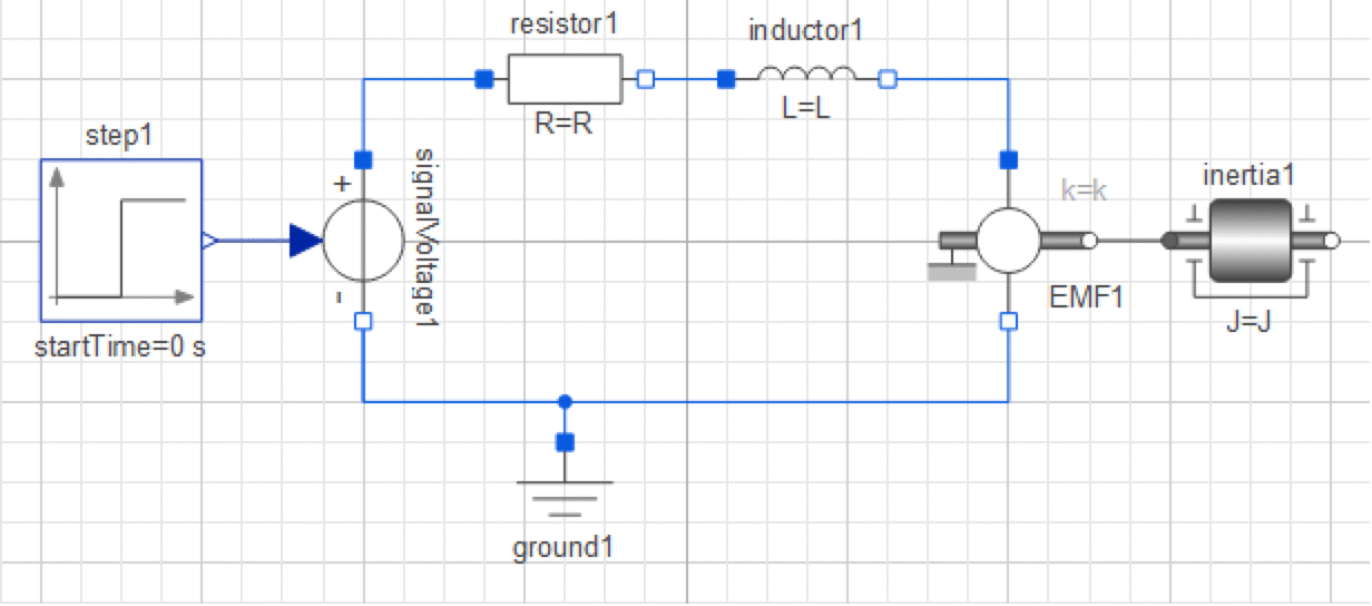
The Diagram View of a DC motor in Model Center.
To build this model, we need to create a new model, find the appropriate components, drag and drop the components into the diagram area, and finally connect the components using the Connection Line Tool.
We begin by creating a new model with the name DCMotor. To locate the components in the Modelica Standard Library, we can either search for them or, if we know their exact location, open the package that contains them in the Class Browser. We will show how to do both.
To locate the Step source component, we will use the Class Browser to search for it. Type step in the text box of the Class Browser and wait until the results appear.
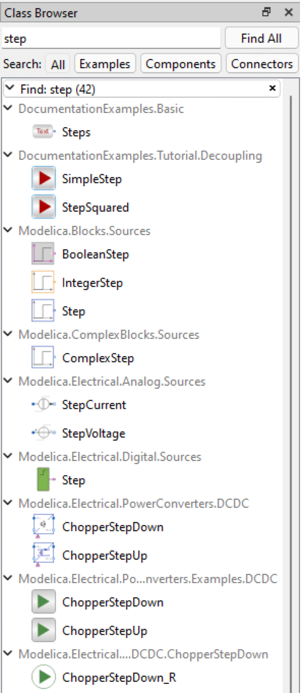
Searching for a step source component using the Class Browser in Model Center.
You should see the top 10 matches for "step" in the Class Browser. The component we want to use is the Modelica.Blocks.Sources.Step component, highlighted in the figure above.
To add this component to our DCMotor model, drag it from the Class Browser and drop it on the Diagram View of the class window.
The signal voltage component is located in the Modelica.Electrical.Analog.Sources package. As we know the exact location of the component, we will use the tree view of the Class Browser and expand the branches of the tree all the way down to the branch that represents the package Sources, in which the component is located.
Start by expanding the Modelica package. This is done by clicking the symbol to the left of the package icon and name.
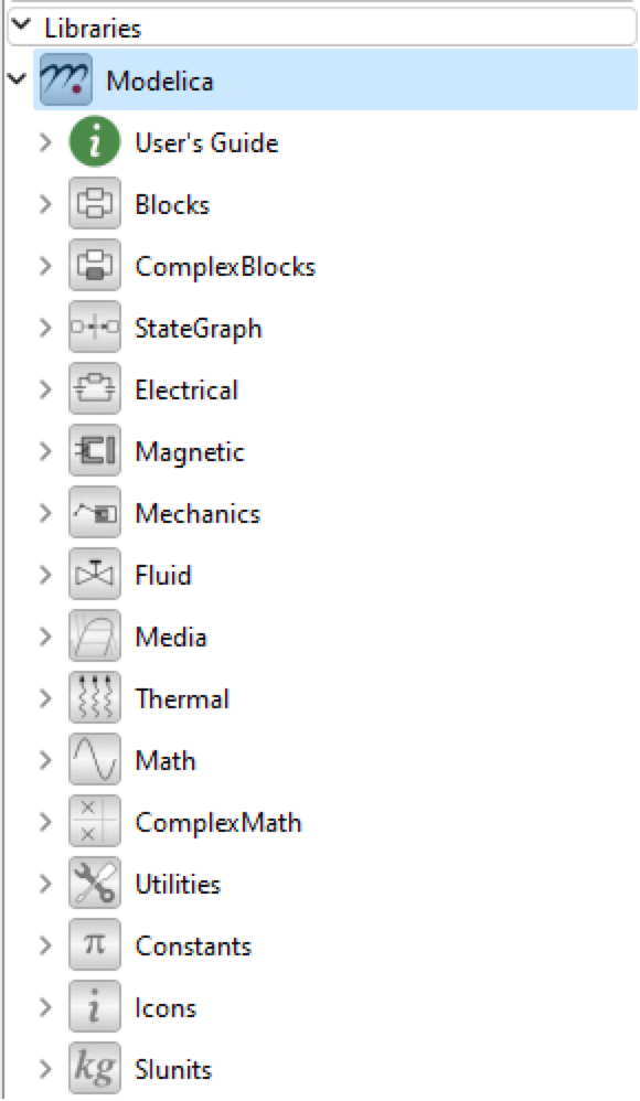
Expanding the Modelica package in the Class Browser.
As you can see, the Modelica package contains several packages. We will continue by expanding the Electrical package, followed by the Analog package, and finally the Sources package, in which we will find the signal voltage component.
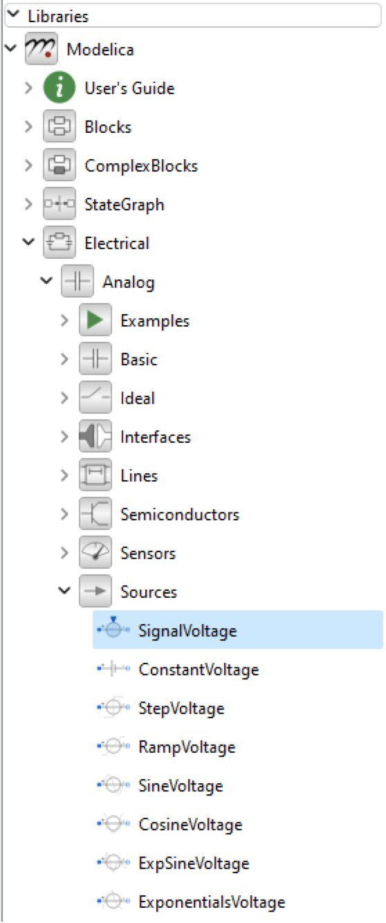
Expanding the Modelica.Electrical.Analog.Sources package.
Add the SignalVoltage component to the DCMotor by dragging it to the Diagram View of the class window.
We have now added two of the seven components. The remaining four electrical components (Resistor, Inductor, Ground, and RotationalEMF) are all found in the Modelica.Electrical.Analog.Basic package. As we already have the Modelica.Electrical.Analog package expanded, we can easily locate the Basic package and expand it in order to find the remaining components.
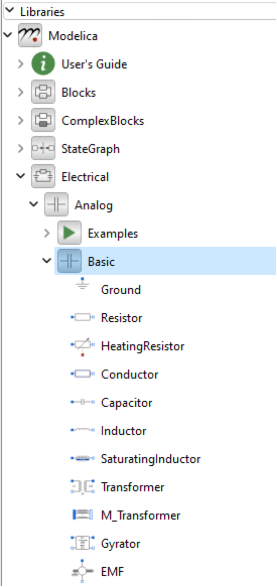
Expanding the Modelica.Electrical.Analog.Basic package.
When you have added the electrical components to the DCMotor model, there is only one component left to add, the inertia. It is located in the Modelica.Mechanics.Rotational.Components package. You can choose if you want to search for it or browse to it directly by expanding the Modelica, Mechanics, Rotational, and Components packages.
Once you have added the inertia component, all that remains to complete the model of the DC motor is to connect the components. Components are connected using the Connection Line Tool.
![]()
The Connection Line Tool in the toolbar of Model Center.
For instance, to connect the ground to the negative pin of the signal voltage component, place the mouse cursor above the ground pin, press the left mouse button, and hold it down while moving the mouse cursor to the negative pin of the signal voltage component. To make the connection, release the mouse button.
Continue connecting all the components until the Diagram View of the DCMotor resembles the first figure in this tutorial.
While dropping and connecting the components, Model Center generates the Modelica code corresponding to the actions. Switch to the Modelica Text View to view the textual representation of the model. In the textual representation of the model, each component is declared, and each connection between two components is represented by a connect equation in the equation section.
model DCMotor
  Modelica.Blocks.Sources.Step step1;
  Modelica.Electrical.Analog.Basic.Resistor resistor1;
  Modelica.Electrical.Analog.Basic.Inductor inductor1;
  Modelica.Electrical.Analog.Basic.RotationalEMF EMF1;
  Modelica.Electrical.Analog.Basic.Ground ground1;
  Modelica.Electrical.Analog.Sources.SignalVoltage signalVoltage1;
  Modelica.Mechanics.Rotational.Components.Inertia inertia1;
equation
  connect(resistor1.n, inductor1.p);
  connect(inductor1.n, EMF1.p);
  connect(step1.y, signalVoltage1.v);
  connect(signalVoltage1.p, resistor1.p);
  connect(EMF1.n, signalVoltage1.n);
  connect(ground1.p, signalVoltage1.n);
  connect(EMF1.flange, inertia1.flange_a);
end DCMotor;
The order of the declarations and equations depends on the order in which components were dropped and connections were made. Therefore, the order of the declarations and equations may be slightly different in your model. Also, for readability, all graphical annotations represented by the » character in an actual Modelica Text View have been removed from the definition of the DCMotor above.
The DCMotor model is now complete and possible to simulate. First, however, we want to specify certain simulation settings. Click the down arrow next to the Simulate Class button in the toolbar and choose Experiment Setup. In the Class Properties dialog box that pops up, set the simulation time to 25 seconds by editing the Stop time. Clicking OK or pressing Return will apply the settings to the model and automatically update the model's experiment annotation. Now click the Simulate Class button in the toolbar to open Simulation Center and simulate the model.
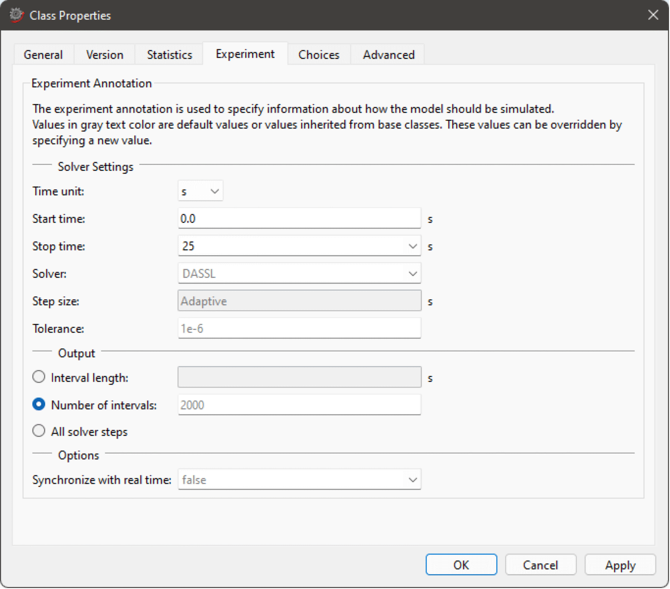
Setting the simulation time to 25 seconds for the DCMotor model.
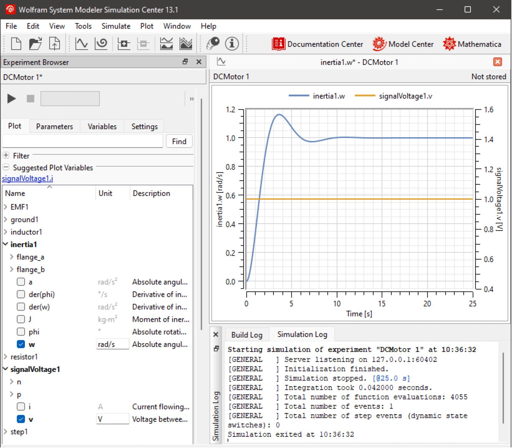
Select the variables to plot in the Experiment Browser as illustrated in the figure below.
Plotting inertia1.w and signalVoltage1.v for the DCMotor model with default parameter values.
Finally, we get the result, with the plot of inertia1.w and signalVoltage1.v versus time.
It is also easy to change parameter values in order to modify the system behavior. We will change the resistance of the resistor, the inductance of the inductor, and the moment of inertia of the axis in order to yield a damped step response instead of an oscillative step response.
Switch to the Parameters view in the Experiment Browser. To edit a parameter value in the Parameters view, click the current value. Set the resistance R of resistor1 to 10 ohm, the inductance L of inductor1 to 0.1 H, and the moment of inertia J of inertia1 to 0.3 kgm 2.
Simulate the model again and study the updated plot of the angular velocity of the inertia.
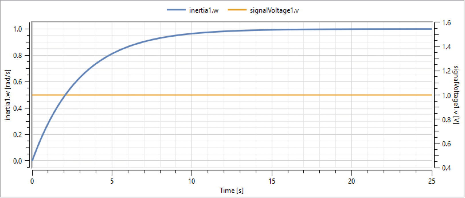
Plotting inertia1.w and signalVoltage1.v for the DCMotor model with customized parameter values.
Stiff and Weak Axis
In this section we will begin by developing a stiff axis model, study its step response by adding a step torque as illustrated below, and show how the axis can be more accurately modeled by including an additional weakness to the stiff axis model.
We begin by developing the stiff axis model. The components (Step, Torque, Inertia, and IdealGear) of the model can all be found by expanding the Modelica.Blocks.Sources, Modelica.Mechanics.Rotational.Sources, and Modelica.Mechanics.Rotational.Components packages in the Class Browser, or by simply searching for them. You can give the model any name you want. The different stages of the model are also available in the IntroductoryExamples.MultiDomain package.

The Diagram View of the IntroductoryExamples.MultiDomain.StiffAxis model.
By selecting the idealGear1 component, we are able to edit the parameters of the component in the Parameters view, located at the bottom part of the editor.
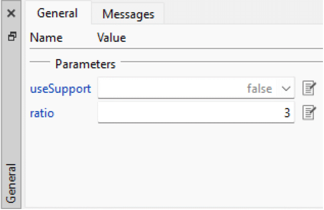
Editing the transmission ratio of an ideal gear component in Model Center.
Give the ratio parameter a value of 3. This means that angles and angular velocities are amplified three times and the torque is attenuated by a factor of three from one side of the gear to the other. Also, change the start time of the step source by changing the value of the parameter startTime to 1 second.
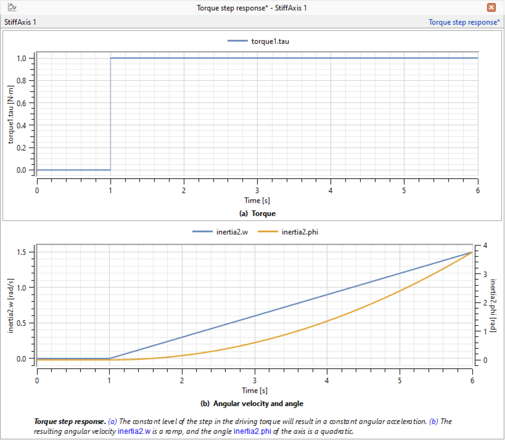
After simulating the system for 6 seconds, we observe that a constant torque results in a constant angular acceleration, i.e. a ramp in angular velocity and a square curve for the angle of the axis, as seen below.
Plotting the torque, the angular velocity of inertia2, and the angle of inertia2 for the IntroductoryExamples.MultiDomain.StiffAxis model.
By including an additional weakness, the axis can be more accurately modeled. This is possible by substituting the above axis model with a model consisting of two rotating masses connected by a torsion spring, according to the figure below. The torsion spring is found in the Modelica.Mechanics.Rotational.Components package.

The Diagram View of the IntroductoryExamples.MultiDomain.WeakAxis model.
Component inertia1 has been given a moment of inertia of 1 kg·m 2, whereas inertia2 and inertia3 have moments of inertia of 0.5 kg·m 2. The spring constant of spring1 is set to 5 N·m/rad. We will simulate this subsystem for 6 seconds and study the result (see below). Note that inertia3, and not inertia2 as earlier, is the last element of the axis, and is therefore the selected plot variable.
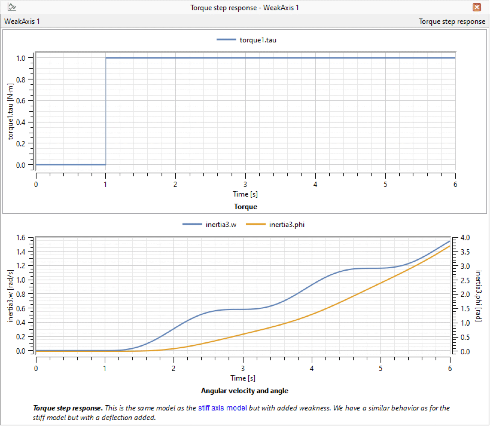
Plotting the torque and the angle of inertia3 (upper plot) and the angular velocity of inertia3 (lower plot) for the IntroductoryExamples.MultiDomain.WeakAxis model.
A comparison between the weak axis model and the stiff axis model shows that they behave similarly, but the former has an added deflection.
Exercise
Make a simple DC motor with a torsion spring to the outgoing shaft and another inertia element. Simulate and study the results. Adjust some parameters and compare results. You may also want to add an input torque and connect it to inertia2, then study the system.
Control System
As the next step of this tutorial, we develop a stiff and weak servo mechanism using the DC motor model and axis models developed above.
The structure of the control system is shown in the schematic picture below. This system consists of an input signal, a sensor, a feedback loop, and a regulator. The physical system consists of the DC motor and one of the axis systems. Since the physical system has negative static gain, the PI gain must also be negative.

Simplified representation of a control system.
We connect all three subsystems as seen in the figure above. The default choices of regulator parameters are k = 1 and T=1, where the PI regulator transfer function is
We begin by developing a control system for the DC motor and the stiff axis developed earlier. As seen in the figure below, three new components are introduced: a feedback component, a PI controller, and a speed sensor.

The Diagram View of the IntroductoryExamples.MultiDomain.StiffServoMechanism model.
These components can be found in the following packages:
- The PI controller is found in Modelica.Blocks.Continuous.
- The feedback component is found in Modelica.Blocks.Math.
- The speed sensor is found in Modelica.Mechanics.Rotational.Sensors.
When simulating this model, we will pay attention to the response in angular velocity of both the motor axis and the gear axis shown in the figure below. The model was simulated for 25 seconds.
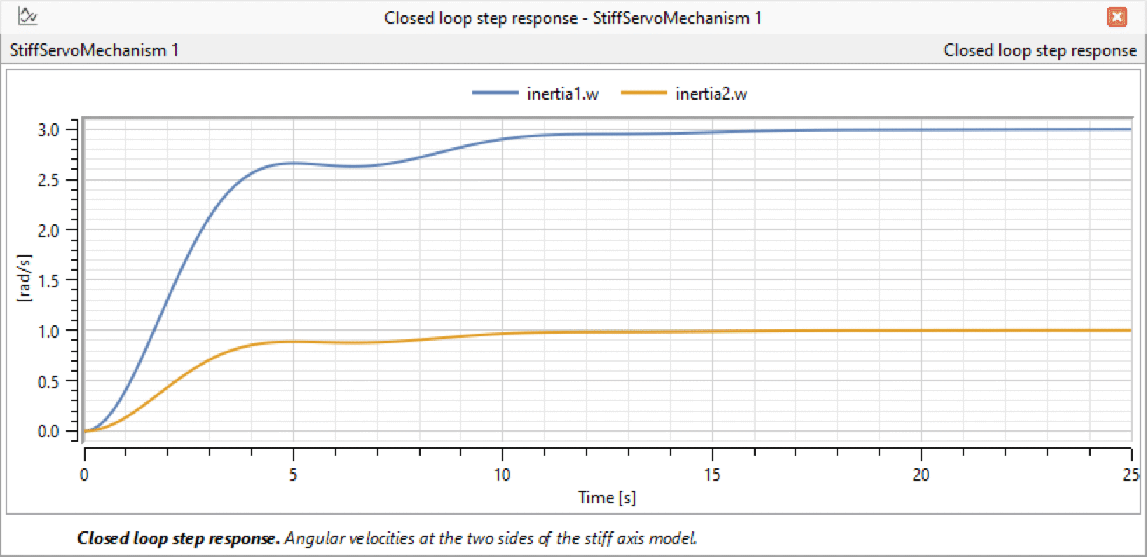
Plotting the angular velocity of inertia1 and inertia2 for the IntroductoryExamples.MultiDomain.StiffServoMechanism model.
Until now we have used default parameters for the controller. By varying the controller gain k, we can control the response. In this case, we vary the gain from 1 to 2 by intervals of 0.25. We can compare the results of all the simulations by creating a new experiment for each simulation and then plotting the results in the same window. New experiments are created by choosing New from the File menu in Simulation Center. Set the appropriate parameter values for each experiment, simulate, and plot the results.
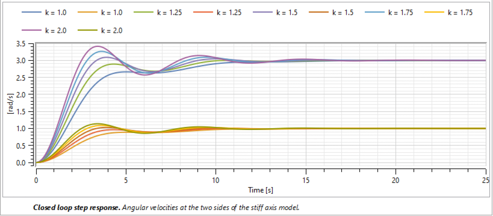
Plotting the angular velocity of inertia1 and inertia2 for the IntroductoryExamples.MultiDomain.StiffServoMechanism model with different controller gain.
By studying the angular velocity response for the motor and gear axes using different regulator gains, we conclude that by choosing k=1.5 we get a sufficiently fast response with few oscillations.
Finally, we develop a control system for the DC motor and the weak axis system.

The Diagram View of the IntroductoryExamples.MultiDomain.WeakServoMechanism model.
Before simulating, we set the controller gain to k=1.5 and compare the results with the results of the stiff axis system.
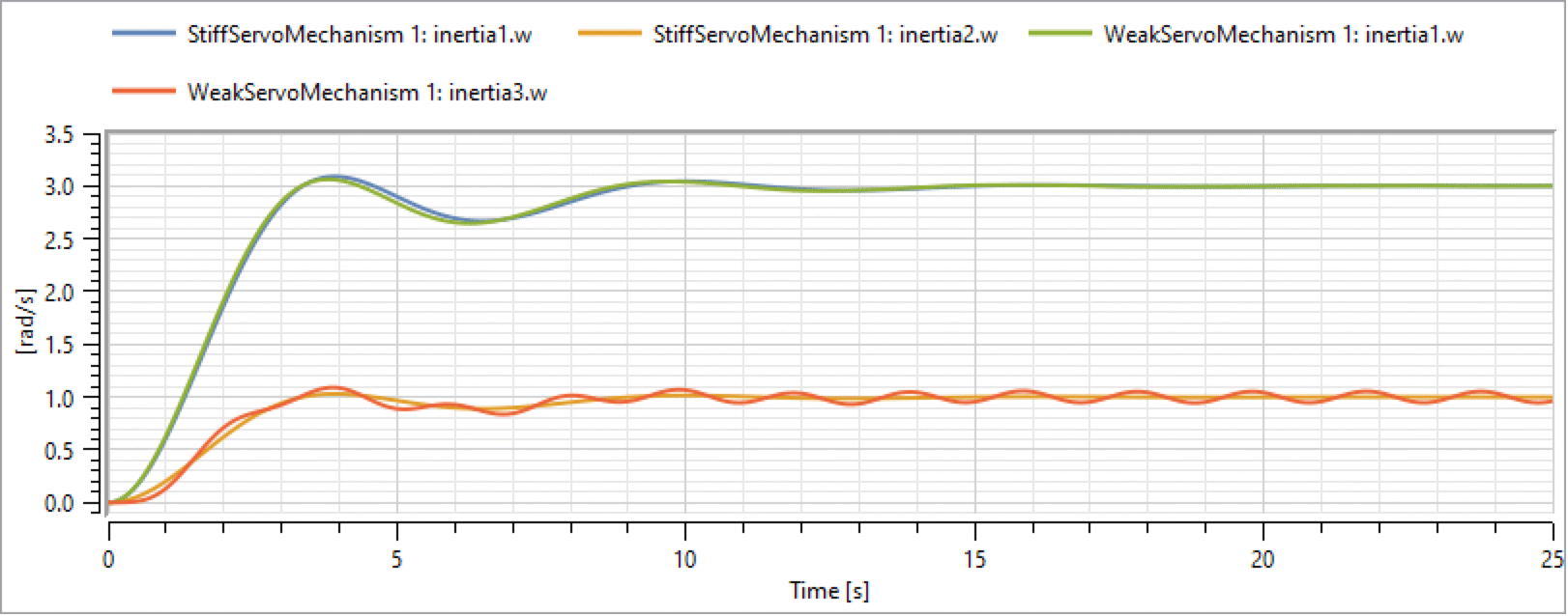
Comparison between the inertias of the StiffServoMechanism model and the WeakServoMechanism model with a regulator gain of k=1.5.
As seen above, the controller design made using the stiff axis model also performs well for the more accurate weak axis.
Sensitivity Analysis
In this section, we will study how sensitive our control design is to changes of different system parameters. This is done using the CVODES solver that supports forward sensitivity analysis. The sensitivity si(t) for a state yi(t) with respect to the parameter p is given by
In other words, at each time instance the sensitivity represents how much the solution for the state yi(t) would change for a small change of parameter p.
Let us study the sensitivity of our control design with respect to the three inertias in WeakServoMechanism. To do so, we select the CVODES solver in the Settings view and check the SA checkboxes in the Parameters view for inertia1.J, inertia2.J, and inertia3.J.
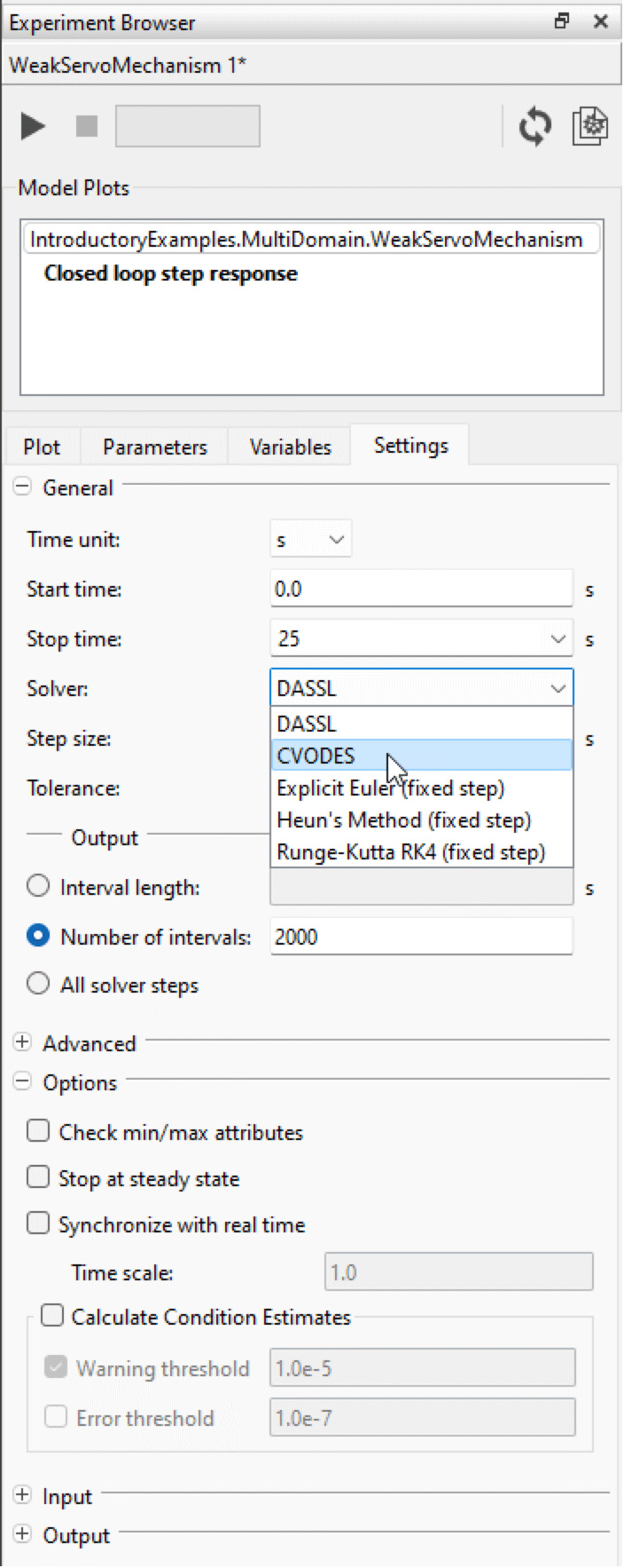
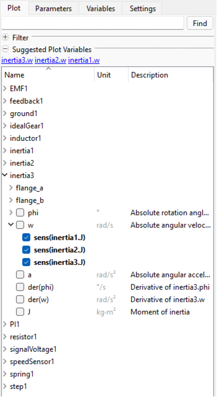
When the simulation has finished, we can plot the result of the sensitivity analysis by clicking the checkboxes in the expandable tree below each state.
Click the checkboxes to plot the sensitivity of inertia3.w with respect to inertia1.J, inertia2.J, and inertia3.J.
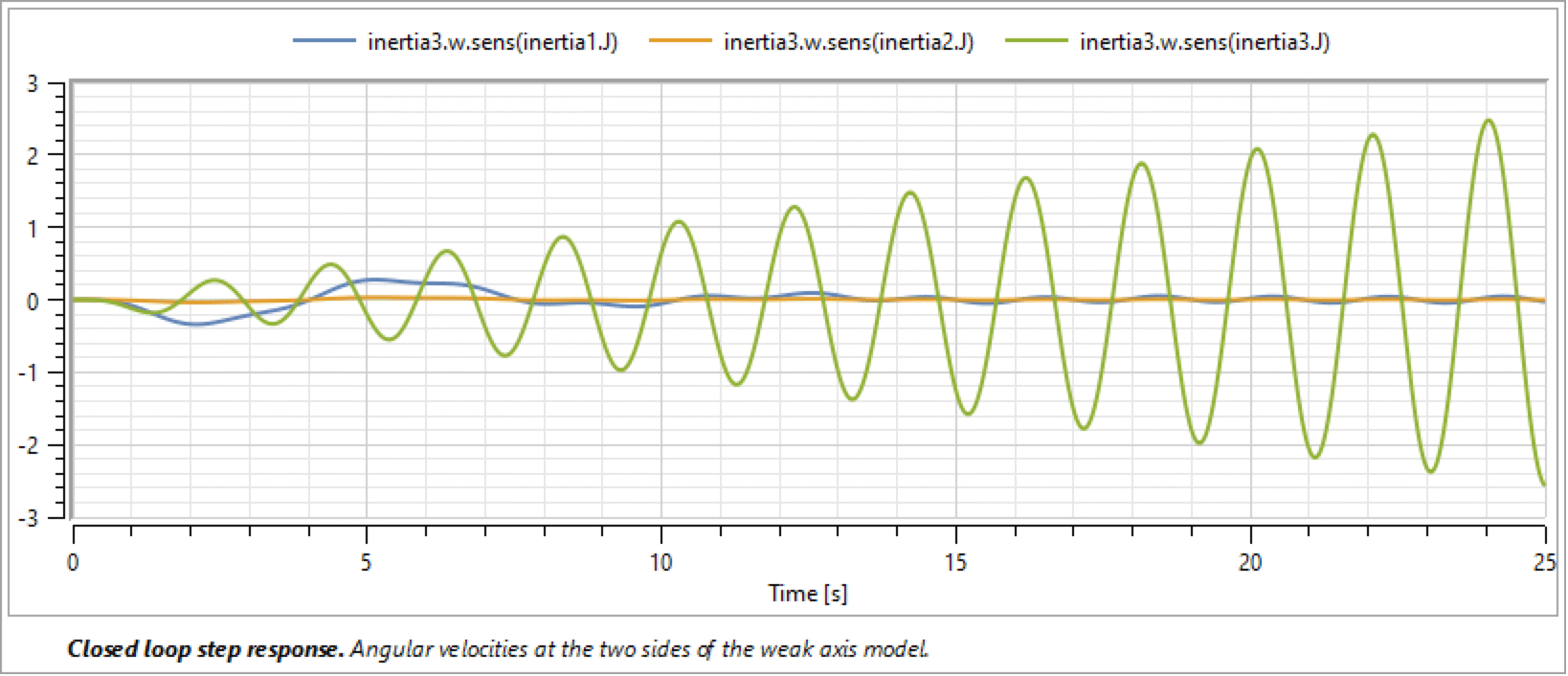
The screen shot below shows the sensitivities for inertia3.w with respect to inertia1.J, inertia2.J, and inertia3.J. There we can see that inertia1.J has a minor impact on the solution of inertia3.w at the beginning of the simulation. This impact diminishes toward the end of the simulation. Furthermore, inertia2.J has a negligible impact on the solution during the whole simulation. inertia3.J, on the other hand, has a significantly larger impact on the solution. From this we can conclude that our control design is most sensitive to changes of inertia3.J.
The sensitivity of inertia3.w with respect to inertia1.J, inertia2.J, and inertia3.J.
To verify our results, we perform the following simulations:
- WeakServoMechanism 2: changing inertia1.J has some impact at the beginning of the simulation, but it diminishes toward the end.
- WeakServoMechanism 4: changing inertia3.J has the most impact; it leads to a phase shift of the oscillations as well as increased amplitude.
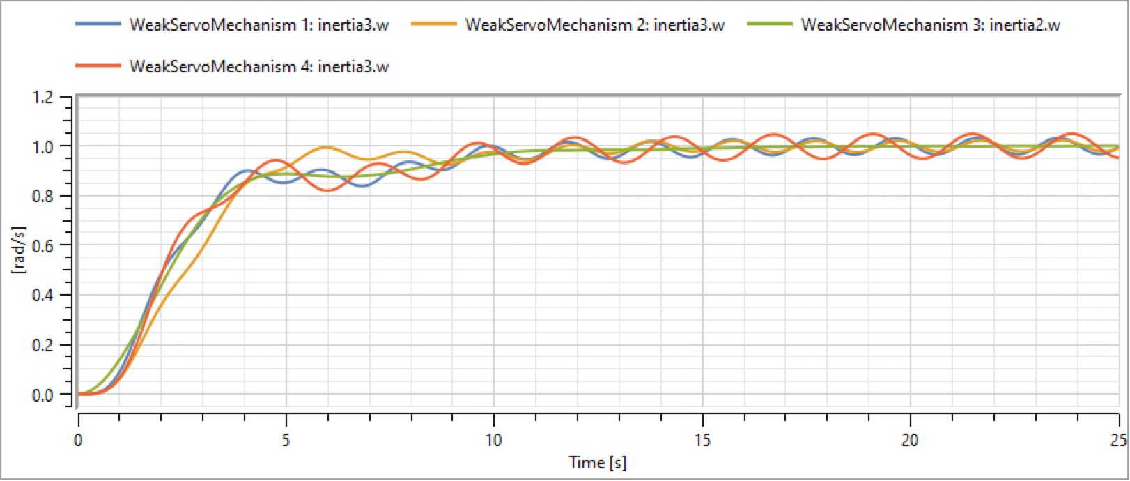
The result of changing inertia1.J, inertia2.J, or inertia3.J.

