|
3.11.3 ApproximateMatrixEquation
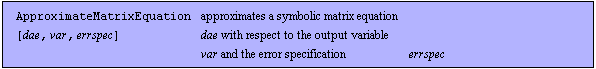
Command structure of ApproximateMatrixEquation.
The function ApproximateMatrixEquation approximates a linear symbolic matrix equation by discarding insignificant matrix entries before the system is solved (simplification before generation, SBG). The significance of a symbolic matrix entry is determined by calculating its numerical influence on the magnitude of the transfer function in one or several frequency sampling points. The approximation process follows a term ranking obtained by computing the large-change sensitivities of the output variable with respect to all matrix entries and sorting the resulting list by least influence. The algorithm deletes all matrix entries whose cumulative influence is less than the user-specified error bound. The error specification errspec has to be given in the following form:
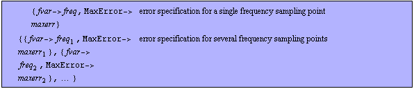
Format for sampling point and error specifications.
For a given errspec, the algorithm assures that the relative magnitude deviation of the output variable var measured at the frequency points fvar =  is less than is less than  . .
ApproximateMatrixEquation has the following options:
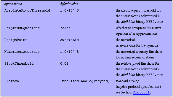
Options for ApproximateMatrixEquation, Part I.

Options for ApproximateMatrixEquation, Part II.
See also: ApproximateTransferFunction.
Options Description
A detailed description of all ApproximateMatrixEquation options is given below in alphabetical order:
AbsolutePivotThreshold
With AbsolutePivotThreshold -> posreal you can specify the minimum absolute value a matrix entry must have to be considered as a pivot candidate during LU decomposition. There is no need to change the value of this option unless ApproximateMatrixEquation reports problems with ill-conditioned equations.
CompressEquations
The setting CompressEquations -> True causes the matrix equation to be compressed after approximation. The option is realized by an internal call of the function CompressMatrixEquation. You should turn matrix compression on whenever you are working with large matrices, i.e. when the matrix dimensions are significantly larger than  . .
DesignPoint
With DesignPoint -> { -> ->  , ,  } you can overwrite the design point given in the DAEObject. The default setting is DesignPoint -> Automatic, which means to use the design point stored in the DAEObject. } you can overwrite the design point given in the DAEObject. The default setting is DesignPoint -> Automatic, which means to use the design point stored in the DAEObject.
NumericalAccuracy
The option NumericalAccuracy -> posreal specifies the minimum influence a matrix entry must have to trigger a recomputation of the term ranking. This threshold is used to prevent frequent ranking recomputations due to numerical inaccuracies in very small influence values.
If the ranking is recomputed too often at the beginning of the approximation process, you should increase the value of NumericalAccuracy by an order of magnitude. Note that information about ranking recomputations is available only if UseExternals -> False and Protocol -> Notebook.
See also the description of RecomputationThreshold.
PivotThreshold
With PivotThreshold -> posreal you can specify the minimum relative magnitude a matrix entry must have to be considered as a pivot candidate during LU decomposition. The value posreal must be a number between  and and  . If it is . If it is  , then the pivoting method becomes complete pivoting, which is very slow and tends to fill up the matrix. If it is set close to zero, the pivoting method becomes strict Markowitz with no threshold. There is no need to change the value of this option unless ApproximateMatrixEquation reports problems with ill-conditioned equations. , then the pivoting method becomes complete pivoting, which is very slow and tends to fill up the matrix. If it is set close to zero, the pivoting method becomes strict Markowitz with no threshold. There is no need to change the value of this option unless ApproximateMatrixEquation reports problems with ill-conditioned equations.
Protocol
This option describes the standard Analog Insydes protocol specification (see Section 3.14.5). Note that detailed protocol information is not available if UseExternals -> True.
QuasiSingularity
QuasiSingularity -> posreal specifies a threshold value for determining whether a matrix is numerically singular. In case the matrix approximation function returns a singular matrix, increase the value of QuasiSingularity by one or several orders of magnitude.
RecomputationThreshold
RecomputationThreshold -> posreal specifies a factor for determining whether the current term ranking should be recomputed. For example, a value of  means that a ranking recomputation is triggered if the true influence of a matrix entry at the current approximation step turns out to be two times larger than predicted initially. Ranking recomputations are triggered only by influence values greater than the value of NumericalAccuracy. means that a ranking recomputation is triggered if the true influence of a matrix entry at the current approximation step turns out to be two times larger than predicted initially. Ranking recomputations are triggered only by influence values greater than the value of NumericalAccuracy.
SortingMethod
The option SortingMethod specifies how the list of matrix entry influences is sorted to obtain a term ranking.

Values for the SortingMethod option.
With the default setting SortingMethod -> PrimaryDesignPoint, the influence list is sorted by influence on the solution of the matrix equation at the first sampling point specified in errspec. The setting SortingMethod -> LeastMeanInfluence causes the least to be sorted by average influence on the solutions at all sampling points.
The setting of the SortingMethod option is relevant only if you specify more than one sampling point. In general, SortingMethod -> LeastMeanInfluence is the preferred setting for multiple sampling points.
StripIndependentBlocks
With StripIndependentBlocks -> True, clusters of equations which are decoupled from the variable of interest, are searched for and discarded after approximation. This option is effective only in conjunction with the setting CompressEquations -> True.
UseExternals
The setting UseExternals -> True causes the MathLink application MSBG.exe to be used for matrix approximation. This is the recommended setting for all platforms for which native Analog Insydes versions exist. You can set UseExternals -> False to run Analog Insydes on other platforms or for debugging purposes in conjunction with the option Protocol. Alternatively, you can also load and unload the module manually as described in Section 3.13.3. For more information refer to UseExternals.
Examples
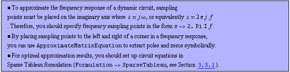
In the following we approximate the system of nodal equations representing the small-signal equivalent circuit of the common-emitter amplifier with respect to the output variable V$5. To obtain an approximation of the amplifier's passband voltage gain, we select a sampling frequency of  . At the sampling point we allow the magnitude of the solution of the approximated equations to deviate from the original design-point value by . At the sampling point we allow the magnitude of the solution of the approximated equations to deviate from the original design-point value by  . .
Load Analog Insydes.
In[1]:= <<AnalogInsydes`
Define an AC model for BJTs.
In[2]:= Circuit[
Model[
Name -> BJT,
Selector -> AC,
Scope -> Global,
Ports -> {B, C, E},
Parameters -> {Rbe, Cbc, Cbe, beta, Ro,
RBE, CBC, CBE, BETA, RO},
Definition -> Netlist[
{CBE, {B, E}, Symbolic -> Cbe, Value -> CBE},
{RBE, {X, E}, Symbolic -> Rbe, Value -> RBE},
{CBC, {B, C}, Symbolic -> Cbc, Value -> CBC},
{CC, {B, X, C, E},
Symbolic -> beta, Value -> BETA},
{RO, {C, E}, Symbolic -> Ro, Value -> RO}
]
]
] // ExpandSubcircuits;
This netlist describes a common-emitter amplifier.
In[3]:= ceamplifier =
Circuit[
Netlist[
{V1, {1, 0}, 1},
{V0, {6, 0}, 0},
{C1, {1, 2}, Symbolic -> C1, Value -> 1.0*^-7},
{R1, {2, 6}, Symbolic -> R1, Value -> 1.0*^5},
{R2, {2, 0}, Symbolic -> R2, Value -> 47000.},
{RC, {6, 3}, Symbolic -> RC, Value -> 2200.},
{RE, {4, 0}, Symbolic -> RE, Value -> 1000.},
{C2, {3, 5}, Symbolic -> C2, Value -> 1.0*^-6},
{RL, {5, 0}, Symbolic -> RL, Value -> 47000.},
{Q1, {2 -> B, 3 -> C, 4 -> E},
Model -> BJT, Selector -> AC,
CBE -> 30.*^-12, CBC -> 5.*^-12, RBE -> 1000.,
RO -> 10000., BETA -> 200.}
]
]
Out[3]= 
Set up a system of symbolic AC equations.
In[4]:= eqs = CircuitEquations[ceamplifier,
ElementValues -> Symbolic]
Out[4]= 
Compute the complexity estimate.
In[5]:= ComplexityEstimate[eqs]
Out[5]= 
Allow for  magnitude error at magnitude error at  . .
In[6]:= errspec = {s -> 2. Pi I 10^4, MaxError -> 0.1}
Out[6]= 
Approximate the system of circuit equations.
In[7]:= sbg = ApproximateMatrixEquation[eqs, V$5, errspec]
Out[7]= 
Estimate the number of terms after approximation.
In[8]:= ComplexityEstimate[sbg]
Out[8]= 
Compute the solution of the approximated equations.
In[9]:= sbgresult = Solve[sbg, V$5]
Out[9]= 
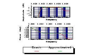
To validate the result, we compute the frequency response of the original system numerically and compare it graphically with the approximated result.
Compute the frequency response numerically.
In[10]:= acsweep = ACAnalysis[eqs, V$5, {f, 1, 1.0*^9}]
Out[10]= 
Evaluate the approximated expression numerically.
In[11]:= sbgn = V$5 /. First[sbgresult] /. GetDesignPoint[eqs]
Out[11]= 
Note that the approximated expression is valid only within the passband because we did not specify sampling points at low or high frequencies.
Plot the exact and approximated functions together.
In[12]:= BodePlot[acsweep, {V$5[f], sbgn},
{f, 1, 1.0*^9}, TraceNames -> {"Exact", "Approximated"}]
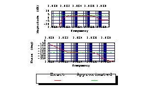
Out[12]= 
Below, we specify a second sampling point at  to extend the validity region of the approximation to low frequencies. Note that you may use a different error bound for each sampling point. to extend the validity region of the approximation to low frequencies. Note that you may use a different error bound for each sampling point.
Add a second sampling point at  . .
In[13]:= errspec2 = {errspec, {s -> 2. Pi I, MaxError -> 0.3}}
Out[13]= 
Approximate the matrix equation.
In[14]:= sbg2 = ApproximateMatrixEquation[eqs, V$5, errspec2,
SortingMethod -> LeastMeanInfluence]
Out[14]= 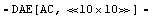
Estimate the number of terms after approximation.
In[15]:= ComplexityEstimate[sbg2]
Out[15]= 
Solve the approximated equations.
In[16]:= sbgresult2 = Solve[sbg2, V$5] // Simplify
Out[16]= 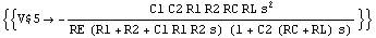
Extract the solution for V$5.
In[17]:= v52 = V$5 /. First[sbgresult2]
Out[17]= 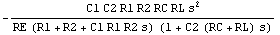
Evaluate the approximated expression numerically.
In[18]:= sbgn2[s_] = v52 /. GetDesignPoint[eqs]
Out[18]= 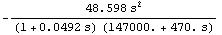
Plot the exact and approximated functions together.
In[19]:= BodePlot[acsweep, {V$5[f], sbgn2[2. Pi I f]},
{f, 1, 1.0*^9}, TraceNames -> {"Exact", "Approximated"}]
Out[19]= 
Note that matrix approximation has reduced the polynomial order of the transfer function from four to two. Therefore, we can now solve the transfer function for the low-frequency poles.
Solve for the low-frequency poles.
In[20]:= Solve[Denominator[v52] == 0, s]
Out[20]= 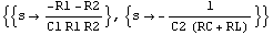
|