|
3.8.6 RootLocusByQZ
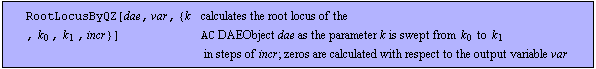
Command structure of RootLocusByQZ.
With RootLocusByQZ you can sweep a parameter of a linear system over an interval and calculate the root locus of the system directly from the corresponding circuit equations using the QZ algorithm. The argument dae has to be an AC DAEObject written in matrix form (see CircuitEquations in Section 3.5.1).
RootLocusByQZ returns data in the following form:
  Poles -> Poles ->  poles poles , Zeros -> , Zeros ->  zeros zeros , ,
SweepParameters ->   -> ->    , ,  
The return value can directly be used as input for RootLocusPlot for visualizing the root locus.
Note that this function is accessible only if the global Analog Insydes option UseExternals is set to True and if a native version of the external MathLink module QZ.exe is available for your machine (see Section 3.13.4).
RootLocusByQZ has the following option:

Option for RootLocusByQZ.
See also: PolesAndZerosByQZ, RootLocusPlot, UseExternals.
Examples
Load Analog Insydes.
In[1]:= <<AnalogInsydes`
Read in a PSpice netlist and small-signal data.
In[2]:= buffer = ReadNetlist[
"AnalogInsydes/DemoFiles/Buffer.cir",
"AnalogInsydes/DemoFiles/Buffer.out",
Simulator -> "PSpice"]
Out[2]= 
Set up system of symbolic AC equations.
In[3]:= mnabuffersym = CircuitEquations[buffer,
AnalysisMode -> AC, ElementValues -> Symbolic]
Out[3]= 
Get the design-point value of Cbc$Q$T5.
In[4]:= Cbc$Q$T5 /. GetDesignPoint[mnabuffersym]
Out[4]= 
Calculate root locus of the circuit as Cbc$Q$T5 is varied from  to to  in steps of in steps of  . .
In[5]:= rloc = RootLocusByQZ[mnabuffersym, V$99,
{Cbc$Q$T5, 5.0*^-12, 50.0*^-12, 5.0*^-12}];
Show the root locus.
In[6]:= RootLocusPlot[rloc, LinearRegionLimit -> Infinity,
PlotRange -> 5.0*^6]
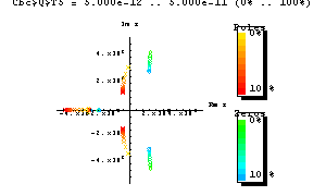
Out[6]= 
|