|
3.8.7 LREigenpair

Command structure of LREigenpair.
As an alternative to the QZ algorithm, Analog Insydes provides the function LREigenpair for solving GEPs iteratively using a variant of the Jacobi orthogonal correction method. This approach is more efficient and reliable than the QZ algorithm for large GEPs when only one single eigenvalue is sought. In addition to the eigenvalue, LREigenpair also yields the corresponding left and right eigenvectors. The argument dae has to be an AC DAEObject written in matrix form (see CircuitEquations in Section 3.5.1).

LREigenpair returns a list of the form {{lambda, v, u,  , ,  , iter}}, where lambda, v, and u denote the calculated eigenvalue and eigenvectors, , iter}}, where lambda, v, and u denote the calculated eigenvalue and eigenvectors,  and and  the corresponding the corresponding  norms of the residual vectors norms of the residual vectors

The last return value, iter, denotes the number of iterations needed to compute lambda with the desired accuracy.
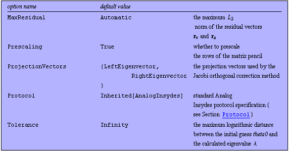
LREigenpair has the following options:

Options for LREigenpair, Part I.

Options for LREigenpair, Part II.
See also: GeneralizedEigensystem.
Options Description
A detailed description of all LREigenpair options is given below in alphabetical order:
AccuracyGoal
AccuracyGoal -> n specifies the desired accuracy of the sought eigenvalue in terms of the number of accurate significant digits. The value of AccuracyGoal is used to determine an appropriate setting for the MaxResidual option if MaxResidual -> Automatic.
DesignPoint
With DesignPoint -> dp, you can specify a list of design-point values for the coefficients of a symbolic system of circuit equations. The default setting DesignPoint -> Automatic causes LREigenpair to use the design-point information stored in dae. You can use the DesignPoint option to override design-point data stored in dae.
FrequencyVariable
LREigenpair needs to know the symbol which represents the complex frequency in order to be able to decompose the system of circuit equations dae into the matrices  and and  . With FrequencyVariable -> Automatic, the symbol is determined automatically from the status information stored in dae. You can specify the frequency variable manually with FrequencyVariable -> var. . With FrequencyVariable -> Automatic, the symbol is determined automatically from the status information stored in dae. You can specify the frequency variable manually with FrequencyVariable -> var.
InitialGuess
With InitialGuess -> {v0, u0}, you can specify initial guesses for the sought eigenvectors  and and  . Both v0 and u0 must be real or complex-valued numeric vectors whose dimensions are compatible with dae. . Both v0 and u0 must be real or complex-valued numeric vectors whose dimensions are compatible with dae.
MaxIterations
MaxIterations -> n specifies the maximum number of orthogonal correction iterations LREigenpair should use in order to find an eigenvalue and the corresponding eigenvectors. If LREigenpair fails to find solutions which satisfy the MaxResidual specification within  iterations, a warning is generated and the most recent iterates are returned. iterations, a warning is generated and the most recent iterates are returned.
MaxResidual
With MaxResidual -> maxres, you can set the convergence criterion for LREigenpair. The value maxres denotes the maximum  norm the residual vectors norm the residual vectors  and and  may have such that the current set of iterates can be regarded as valid approximations of the sought eigenpairs. LREigenpair stops iterating as soon as both may have such that the current set of iterates can be regarded as valid approximations of the sought eigenpairs. LREigenpair stops iterating as soon as both  and and  fall below maxres. fall below maxres.
With the default setting MaxResidual -> Automatic, the maximum residual norm is computed as

Note that the value of maxres depends on the setting of the Prescaling option because the norms of  and and  are computed after prescaling. are computed after prescaling.
Prescaling
With Prescaling -> True, LREigenpair scales the rows of the matrix pencil  such that the absolute value of the largest coefficient in each row is 1. In general, prescaling improves the numerical properties of ill-conditioned GEPs and helps to reduce the number of iterations. Prescaling does not change the eigenvalues and eigenvectors of the matrix pencil. You can turn off prescaling by setting Prescaling -> False. such that the absolute value of the largest coefficient in each row is 1. In general, prescaling improves the numerical properties of ill-conditioned GEPs and helps to reduce the number of iterations. Prescaling does not change the eigenvalues and eigenvectors of the matrix pencil. You can turn off prescaling by setting Prescaling -> False.
ProjectionVectors
Starting with a given initial guess  for the sought eigenvalue and eigenvectors, LREigenpair repeatedly solves the correction equation for the sought eigenvalue and eigenvectors, LREigenpair repeatedly solves the correction equation

for updates  of of  and and  . The symbols . The symbols  and and  denote two arbitrary projection vectors, which must be chosen appropriately in each step to ensure convergence of the iterates. Suitable choices for denote two arbitrary projection vectors, which must be chosen appropriately in each step to ensure convergence of the iterates. Suitable choices for  and and  include combinations of the initial guesses and the most recent approximations of the eigenvectors include combinations of the initial guesses and the most recent approximations of the eigenvectors  and and  . .
With the option ProjectionVectors -> {wt, yt}, you can choose the vectors LREigenpair uses as projection vectors. Possible values are:

Values for the ProjectionVectors option.
In most cases, the default setting ProjectionVectors -> {LeftEigenvector, RightEigenvector} constitutes an appropriate choice. You will need to change the setting of this option only if you encounter convergence problems.
Tolerance
Tolerance -> tol specifies the radius of the tolerance region around the initial guess theta0 in which the sought eigenvalue  should lie. LREigenpair generates a warning if it converges to an eigenvalue that lies outside the tolerance region. The Tolerance option allows you to check whether LREigenpair has found the eigenvalue you wished to compute or whether the iterations have converged to a completely different solution. should lie. LREigenpair generates a warning if it converges to an eigenvalue that lies outside the tolerance region. The Tolerance option allows you to check whether LREigenpair has found the eigenvalue you wished to compute or whether the iterations have converged to a completely different solution.
Tolerance uses a logarithmic measure for distances. For example, Tolerance -> 1.0 allows the value of the solution  to lie within to lie within  and and  times the value of the initial guess theta0. times the value of the initial guess theta0.
Examples
Load Analog Insydes.
In[1]:= <<AnalogInsydes`
Define three square real-valued matrices.
In[2]:= A = {{1, 2}, {-3, 1}};
B = {{1, 4}, { 2, 1}};
B2 = {{1, -1}, {0, 0}};
Solve the GEP  iteratively using the initial guess iteratively using the initial guess  . .
In[3]:= LREigenpair[A, B2, -3.0]
Out[5]= 
Solve the GEP  . Specify initial guesses for the eigenvectors. . Specify initial guesses for the eigenvectors.
In[4]:= LREigenpair[A, B, -1., InitialGuess -> {{0, 1}, {1, 0}}]
Out[6]= 
Use the default projection vectors.
In[5]:= LREigenpair[A, B, 1., MaxResidual -> 1.*^-15]
Out[7]= 
Note that the following setting for ProjectionVectors increases the number of iterations.
Use right eigenvectors as projection vectors.
In[6]:= LREigenpair[A, B, 1., MaxResidual -> 1.*^-15,
ProjectionVectors ->
{RightEigenvector, RightEigenvector}]
Out[8]= 
The setting Tolerance -> 1.0 allows the value of the solution  to lie within to lie within  and and  times the value of the initial guess theta0. times the value of the initial guess theta0.
Search for an eigenvalue in the interval 
In[7]:= LREigenpair[A, B, -100., Tolerance -> 1.]

Out[9]= 
With the default setting Tolerance -> Infinity, any solution of the GEP is accepted without a warning.
Do not specify a tolerance region.
In[8]:= LREigenpair[A, B, -100., Tolerance -> Infinity]
Out[10]= 
Read in a PSpice netlist and small-signal data.
In[9]:= buffer = ReadNetlist[
"AnalogInsydes/DemoFiles/Buffer.cir",
"AnalogInsydes/DemoFiles/Buffer.out",
Simulator -> "PSpice"]
Out[11]= 
Set up a system of symbolic AC equations.
In[10]:= mnabuffersym = CircuitEquations[buffer,
AnalysisMode -> AC, ElementValues -> Symbolic]
Out[12]= 
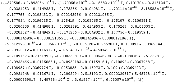
Find the pole of the buffer circuit near  and the corresponding left and right eigenvectors. and the corresponding left and right eigenvectors.
In[11]:= lreigenpairs = LREigenpair[mnabuffersym, 3.0*^6 I]
Out[13]= 
Show the eigenvalue.
In[12]:= lreigenpairs[[1, 1]]
Out[14]= 
Compare the eigenvalue with the result of the QZ algorithm.
In[13]:= Cases[PolesByQZ[mnabuffersym], _Complex]
Out[15]= 
|