2.5.1 Bode Plots

The Bode plot is perhaps the most commonly used graphing scheme for visualizing frequency responses of linear analog systems. It consists of two separate charts which display magnitude and phase of a transfer function on a logarithmic and a linear scale vs. frequency, the latter being scaled logarithmically. The magnitude values are usually given in decibels (dB) and the phase values in degrees.

In Analog Insydes, Bode plots are displayed using the command BodePlot. With the basic syntax

BodePlot[tfunc, frange]

you can plot the transfer function tfunc within the frequency range frange. The transfer function must be a complex-valued function of the frequency variable fvar, and the frequency range a list of the form {fvar, fstart, fend}. BodePlot also allows to plot several transfer functions simultaneously. For this purpose, the first argument of BodePlot must be specified as a list of transfer functions.

BodePlot[, , , frange]

To demonstrate the Bode plot facility we define the following transfer function in terms of the frequency variable s.

In[1]:= <<AnalogInsydes`

In[2]:= H1[s_] := 1000./(1. + 10.1*s + s^2)

We then display a Bode plot of the frequency response by evaluating H1 along the imaginary axis, , for a frequency range of to .

In[3]:= BodePlot[H1[I w], {w, 0.001, 1000.}]

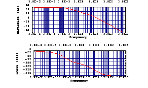
Out[3]=

BodePlot Options

The output generated by BodePlot is influenced by a number of options listed in Options[BodePlot], many of which are inherited from Options[LogLinearListPlot] from Mathematica's standard package Graphics`Graphics`. Here, we will discuss only some of those options which pertain exclusively to BodePlot or which must be used with a different syntax as compared to LogLinearListPlot. The relevant options and their default settings are listed below. Defaults are listed first, followed by the possible alternatives printed in slanted typewriter font.

MagnitudeDisplay -> Decibels | AbsoluteValues | Linear

PhaseDisplay -> Degrees | Radians

PlotRange -> Automatic, Automatic

The option MagnitudeDisplay controls the display of the magnitude values. When set to AbsoluteValues, magnitude values are not converted to decibels. Instead the absolute numerical values are displayed on a logarithmic scale. When MagnitudeDisplay is set to Linear, magnitude values are displayed on a linear scale. In a strict sense, the latter does no longer constitute a true Bode plot, but there exist a few applications where linear magnitude scaling is useful.

With the value of the option PhaseDisplay we can choose whether phase values are shown as degrees or as radians.

The meaning of the PlotRange option is slightly different for BodePlot than for other Mathematica plotting commands. Here, the value of PlotRange must be a list of two elements, {, }, specifying the plot ranges of the -axes of the magnitude and the phase chart respectively. PlotRange has no effect on the ranges of the -axes as these are determined by the given frequency range. The format for both -ranges is the usual one as documented in the Mathematica manual, so any of the forms below are valid syntax:

Automatic

ymin, ymax

ymin, Automatic

Let's graph H1 together with a second transfer function H2 and watch the effects of some BodePlot options. Other common graphics options such as PlotStyle can be applied just as usual.

In[4]:= H2[s_] := 100./(1.6 + 8.2*s + s^2)

In[5]:= BodePlot[{H1[I w], H2[I w]}, {w, 0.001, 1000.},
PhaseDisplay -> Radians,
PlotRange -> {{-60, 80}, Automatic},
PlotStyle -> {{RGBColor[0, 0, 1], Dashing[{0.05}]},
{RGBColor[0, 1, 0]}}]

Out[5]=