2.5.2 Nyquist Plots

Another widely used graphical representation of transfer functions is the Nyquist plot. It is a parametric plot of the real and imaginary part of a transfer function in the complex plane as the frequency parameter sweeps through a given interval. Nyquist plots are particularly useful for stability analysis in control system design because one can immediately check whether a negative feedback loop meets Nyquist's stability criterion: If the Nyquist curve of the open loop system wraps around the point  on the real axis then the corresponding closed loop system is unstable.

Nyquist plots are produced by the command NyquistPlot whose argument sequence is the same as that of BodePlot. Just as in the case of the latter you can plot one single transfer function or several transfer functions simultaneously.

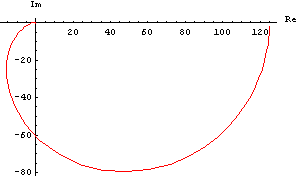
Let's make a Nyquist plot of the frequency response of a system which is formed by a series connection of the two transfer functions H1 and H2, followed by a attenuator (). The overall transfer function of the resulting system is given by the product of the individual transfer functions.

In[6]:= H12a[s_] := H1[s] * H2[s] * 0.002

To make the curve look smoother we increase the number of plot points to .

In[7]:= NyquistPlot[H12a[I w], {w, 0.001, 1000.},
PlotPoints -> 100]

Out[7]=

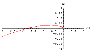
We determine whether the corresponding closed-loop system is stable or unstable by taking a closer look at the region around the point  using the PlotRange option.

In[8]:= NyquistPlot[H12a[I w], {w, 0.1, 1000.},
PlotPoints -> 100, PlotRange -> {{-3, 1}, {-1, 1}}]

Out[8]=

This plot reveals that the point  is located to the right of the Nyquist curve, i.e. the curve wraps around the critical point. Hence the closed-loop system is unstable.

NyquistPlot Options

NyquistPlot inherits its plot options, which are accessible through Options[NyquistPlot], from Mathematica's standard function ListPlot. See the Mathematica book for detailed explanations of these options. NyquistPlot has additional options like, for example FrequencyScaling which controls the spacing of the frequency points at which the transfer function is sampled. FrequencyScaling can be set to Linear or Exponential, resulting in equidistant or exponentially spaced sampling points respectively. The default is Exponential.