10.4 Dynamic Motion SynthesisThis section covers the use of the SolveFree function to numerically integrate the equations of motion built by SetFree, which is done to find the time-domain dynamic motion of underconstrained systems. The FreeSystem objects that contain the equations of motion to be integrated are built using the same procedure that would be used if only the instantaneous free response was desired. Building such FreeSystem objects is covered in Sections 10.2 and 10.3. 10.4.1 Numerical IntegrationNumerical integration with SolveFree. There are several issues that are specifically associated with the numerical solution of the constrained equations of motion generated by MechanicalSystems. The equations of motion are a nonminimal differential-algebraic system of equations, that may or may not be linear in the highest-order terms.
One important issue is constraint violation. The equations of motion do not include the actual kinematic constraints, they only include the second time derivatives of the constraint equations. Because of this, small errors in the numerical integration of the equations of motion can accumulate into large violations of the kinematic constraints and their first derivatives. To deal with this problem, the equations can be algebraically reduced to a minimal set, but this is not generally possible with the type of constraints allowed by Mech. Alternatively, the numerical values of the dependent variables can be corrected as the integration progresses so as to continuously satisfy the constraints. This method is implemented in SolveFree.
Another issue is the transformation of angular velocity and acceleration in 3D models. If a model is built with angular coordinates (the Method -> Angular option in SetSymbols) the first and second derivatives of angular orientation are represented by the angular velocity, omega, and the angular acceleration, alpha. Unfortunately, omega is not the first derivative of the Euler parameters used to represent angular orientation. Thus, a coordinate transformation must occur at each time step to allow the Euler parameters to be integrated. SolveFree handles this transformation automatically, so models built in any coordinate system can be integrated.
The equations of motion are not necessarily linear in their highest-order terms, depending on the form of the applied loads. SolveFree automatically switches to an iterative solution method for nonlinear systems that allows them to be solved, albeit slowly. Initialization OptionsThe only option that is concerned with the initialization of the integrator is the InitialCondition option. All other information needed to integrate the equations of motion is contained in the FreeSystem object. This option is most useful for repeatedly integrating the same FreeSystem with different sets of initial conditions without having to rerun SetFree. An initialization option for SolveFree. The list of rules required by InitialCondition is of the form returned by SolveMech. Using SolveMech to generate the initial conditions (which is essentially what is done by the default setting) guarantees that the initial conditions constitute a valid solution to the constraint equations. If initial conditions that do not satisfy the constraints are passed to SolveFree, the integration will proceed without difficulty, producing results that satisfy the differential equations of motion, but do not satisfy the kinematic constraints.
Note that a sufficient set of initial conditions for integrating a free acceleration system is returned by SolveMech[time, Solution -> Velocity], while a sufficient set of initial conditions for integrating an equilibrium velocity system is returned by SolveMech[time]. Integration OptionsThe following options are used to control the actual integration algorithm used by SolveFree. The default settings for these options are intended to produce reasonable results in the shortest possible time with a well-behaved system. Some tweaking may be required to get the best result from models with large accelerations or force discontinuities. Options for controlling the SolveFree integrator. More options for controlling the integrator. The error estimation used by SolveFree makes an assumption that the approximate magnitude of each of the dependent variables is near to 1. While this assumption is certainly valid for Euler parameters that are between -1 and 1, and the 2D angular coordinate that has units of radians, it is up to the user to choose a system of units such that the linear dimensions of the model are not extremely large or small. While the error estimation routine does not look at the Lagrange multipliers ( 1, 1,  2, ...) it is best to keep the units of force and mass such that the Lagrange multipliers are not extremely large or small, because other parts of the numerical solution method begin to produce significant errors when dealing with a wide range of numerical magnitudes. 2, ...) it is best to keep the units of force and mass such that the Lagrange multipliers are not extremely large or small, because other parts of the numerical solution method begin to produce significant errors when dealing with a wide range of numerical magnitudes.
When step size switching is enabled, SolveFree basically limits the maximum error in any dependent variable at a single time step to be less than the MaxError setting. If this is exceeded at a time step, the integrator backs up, halves the step size, and proceeds forward again. This error limit seems rather loose. If the same variable exhibited the maximum signed error at each time step, the cumulative error in that variable after 1000 time steps would be 0.1! In reality, the large errors occur at discrete points in the motion of a model, so the cumulative error is normally smaller.
The MaxError option can also be used to explicitly specify the error magnitude limits at which the time step size is halved, doubled, or when a corrective versus predictive step is taken. MathError -> {a, b, c} specifies that the time step size will be doubled if the sum of the maximum errors in the last four steps drops below c, it will be halved if the error in the current step goes above a, and an Adams-Moulton corrective step will be taken if the error is between a and b. Thus, MaxError -> {0.0001, 0.00001, 0.000001} is equivalent to the default setting of MaxError -> 0.0001. Iterative Solution OptionsThe following options are used only to control the iterative solution block used for nonlinear models. These options have no effect on linear models. Options for the Newton-Rhapson solution block in SolveFree. Free acceleration models are always linear in the acceleration variables (X2dd, Y3dd, ...) but they may be nonlinear in the Lagrange multipliers ( 1, 1,  2, ... ) if there are loads applied that are algebraically dependent on reaction forces, such as friction. Equilibrium velocity models can be nonlinear in the Lagrange multipliers, and they can also be nonlinear in velocity variables (X2d, Y3d, ...) if the applied loads are nonlinear functions of velocity. The second element in a FreeSystem object tells whether the model is linear or not. FreeSystem[...][[2]] returns True for nonlinear models. 2, ... ) if there are loads applied that are algebraically dependent on reaction forces, such as friction. Equilibrium velocity models can be nonlinear in the Lagrange multipliers, and they can also be nonlinear in velocity variables (X2d, Y3d, ...) if the applied loads are nonlinear functions of velocity. The second element in a FreeSystem object tells whether the model is linear or not. FreeSystem[...][[2]] returns True for nonlinear models. Output Control OptionsThe following options are used to determine what data is returned by SolveFree, and what format is used to returned it. Output options for SolveFree. The StepSize data returned by the Diagnostics setting can be useful to help determine what should be chosen for a constant step size, if one is desired. The MaxError data included by Diagnostics is the measure of error used by the adaptive time step adjustment algorithm to decide when to change the step size. 10.4.2 Planar Example MechanismThe following example uses the pendulum-on-a-rope model that was developed in Section 10.1. The pendulum is released from a constrained zero velocity position, that is not in static equilibrium, and the free response is found.
The spring force that was used to pull the pendulum off to one side is removed from the model, but gravity is retained. Also, nonzero moments of inertia are defined for each body, since the moments of inertia are relevant to the dynamics of the system, while they were not relevant to the equilibrium analysis. This loads the Modeler2D package. Here are the three body objects, including the new inertia properties. The pendulum-on-a-rope model uses seven constraint objects. The constraints that fix the initial position of the model have been altered so that the pendulum may be released from an offset position. Here are the constraints. Here is the gravitational load applied to the pendulum and slider. Now the model is run with SolveMech.
Out[5]= |  |
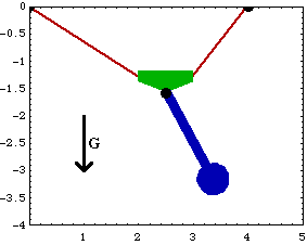
Here is the pendulum-on-a-rope model in its initial configuration.
10.4.3 Free ResponseTo find the free acceleration of the pendulum, a FreeSystem object is built that contains a new set of equations of motion with constraints 5, 6, and 7 dropped from the model. Note that no initial conditions are yet available for the velocity of the bodies in the model. SetFree sets all of the initial velocities to zero if none are specified with the InitialCondition option. This drops the constraints that lock the position of the pendulum. SetFree needs initial conditions for the velocity of each body. Since none are available zero is assumed.

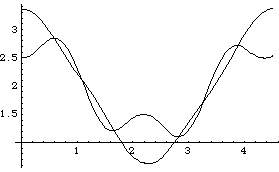
This integrates the FreeSystem object from T = 0 to T = 4.5, which is approximately a full period of the pendulum. The MakeRules option includes the velocity solution in the result. Here is a plot of the X coordinates of the slider and the pendulum.
Out[8]= |  |
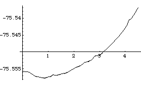
Since the pendulum model is a conservative system, the sum of the kinetic and potential energy in the system should remain constant. This fact can be used to measure the accuracy of the numerical integrator. A special output function. The kinetic energy of each body is given by the BodyEnergy function, and the potential energy is simply the gravitational potential energy mass G altitude. The following plot shows that the numerical error in the integration has allowed the total energy of the model to increase by about 0.04% over 4.5 seconds. Here is the total energy in the pendulum model.
Out[9]= |  |
Tightening the error budget by a factor of 100 by specifying the MaxError -> 0.000001 option for SolveFree will reduce the total energy rise to only 0.0007%, over the same time period, with an associated doubling of run time. Using the ConstraintCorrection -> True option, with the default error budget, will reduce the total energy rise to 0.002% with a slightly smaller increase in run time. In this case, either constraint correction or reducing step size (which is the result of decreasing the error budget) gives similar returns on computer time investment.
Changing the FitDegree setting can also affect the integration error. Setting FitDegree to Quadratic for this example will increase the net energy rise to 0.08%, while setting FitDegree to Quartic will reverse the sign of the error, changing the net energy rise to - 0.04%. Specifying a higher FitDegree setting often produces unexpected results because the automatic time step size adjustment works to counteract the higher degree setting. The integrator measures a smaller error in each step so it chooses a larger step size, resulting in the same net error. Here is the pendulum-on-a-rope model at T = 1, 2, and 3 seconds.

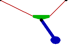
Here is an animation of the pendulum-on-a-rope model.
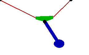
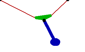
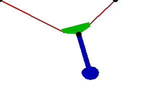
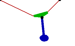
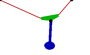
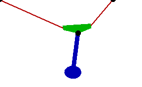
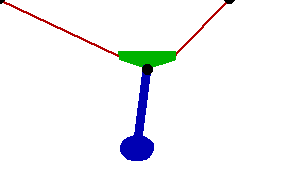
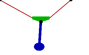
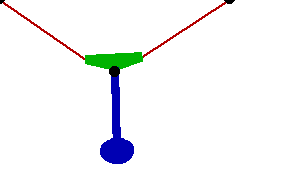
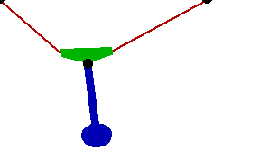
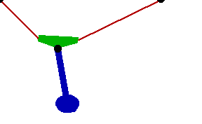
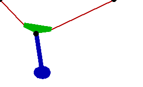
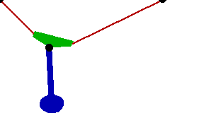
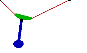
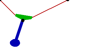
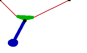
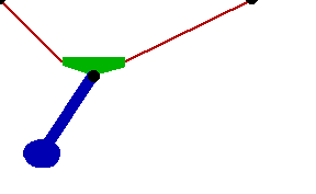
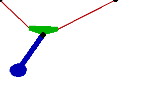
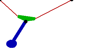
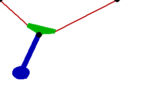
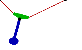
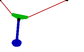
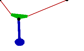
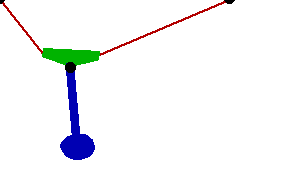
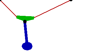
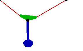
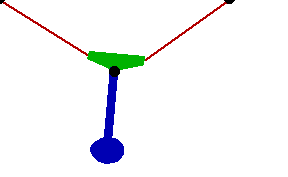
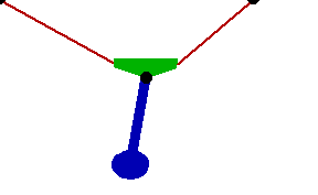
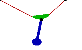
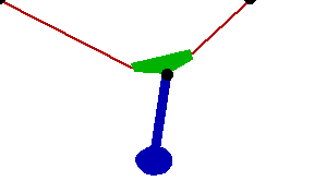
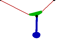
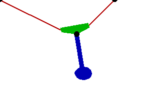
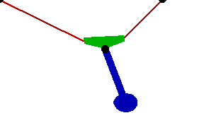
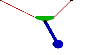
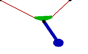
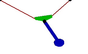
10.4.4 Gyroscopic ExampleThe following example integrates the motion of the gyroscope model that was presented in Section 10.3. The model uses the GyroMoment function, which was also presented in Section 10.3, to reduce the numerical burden of integrating the motion of the rotor. The angular local coordinate system is used, which requires SolveFree to use a coordinate transformation during the integration. This loads the Modeler3D package and defines names for each of the body numbers. Here are the constraints, bodies, and loads for the gyroscope model. The model is run to prepare the initial conditions for SetFree. Note that the rotor has no angular velocity because it is modeled in the GyroMoment load.
Out[20]= |  |
10.4.5 Free ResponseTo find the unconstrained motion of the gyroscope, a FreeSystem object is built that contains a new set of equations of motion with constraints 2, 4, and 6 dropped from the model. Constraint 6, the constraint that locks the rotation of the rotor to that of the gimbal, is dropped in this simulation because the gross motion of the rotor results in some relative angular acceleration between these two bodies. If constraint 6 was not dropped, the model would represent an enforced constant angular velocity between the rotor and the gimbal, as if the rotor had a constant velocity motor attaching it to the gimbal.
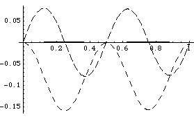
The constant moment that was applied to the base is retained, so the model is expected to gain energy with the passage of time. This drops the constraints that lock the three rotational axes of the gyroscope. This integrates the FreeSystem object from T = 0 to T = endt. The MakeRules option includes the velocity solution in the result. Here is a plot of the three components of the angular velocity of the gimbal. The Z component is simply oscillating about zero, so the applied torque is producing no net motion of the gimbal. The Y component, however, is consistently negative, so the gimbal is precessing in an oscillatory manner.
Out[23]= |  |
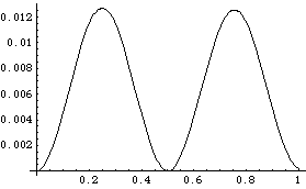
Here is a plot of the rotation angle of the base.
Out[24]= |  |
Note that the Rotation function was not used in the preceding example to resolve the rotation angle of the base from the Euler parameters, but ProjectedAngle was used instead. This was done because the small numerical errors in the integration caused one of the Euler parameters to drift slightly above 1.0. The Euler parameters are not meaningful for absolute values greater than 1, so the Rotation function would return an error. The ProjectedAngle function uses vector algebra, instead of a mathematical identity, and it does not care if the values of the Euler parameters stray above 1.
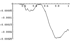
Since the gyroscope model is a conservative system (if the applied moment is recognized as a conservative force) the sum of the kinetic and potential energy in the model should be constant. The potential energy stored by the constant applied moment is the work done by the gyroscope on the applied moment, which is the negative of the magnitude of the applied moment times the is rotation of the base. The following plot shows that the numerical error in the integration has allowed the total energy of the model to decrease by about 2% of the maximum kinetic energy over the integration period. Here is the total energy in the gyroscope, including the energy stored in the constant applied moment.
Out[25]= |  |
This is near to the maximum kinetic energy of the body.
Out[26]= |  |
Tightening the error budget by a factor of 10 with MaxError -> 0.00001 will reduce the total energy rise to only 0.12% over the same period, with an associated increase in run time. Using the ConstraintCorrection -> True option, with the default error budget, will have virtually no effect on the error in the total energy. This is because the error stems from the deviation in the Euler parameters that are very close to 1, an error on which constraint correction has little effect. Using the FitDegree -> Quartic option, with the default error budget, will reduce the total energy rise to 0.71%, with only a small increase in run time. 10.4.6 Reducing Gyroscopic ModelsThere is one more technique that can be applied to 3D gyroscopic models to reduce their size and thereby reduce their run time. This technique can be very useful to models with more than one rotor. A function for modifying an inertia tensor. The restrictions that apply to the use of GyroFilter are identical to the restrictions that apply to the use of GyroMoment. The body represented by the inertia properties must be axially symmetric. The purpose of GyroFilter is to make it possible to add a zero-torque spinning body to a model without actually adding a body to the model at all. To demonstrate, the rotor body is deleted from the previously defined gyroscope model, and replaced with a special load and inertia properties on the gimbal. This time, the model is built in Euler coordinates, just to show that the results are the same. Here is the gyroscope constraint set with the rotor deleted. Here is the body object for the gimbal. It now carries the inertia of what was the rotor with the component in the direction of the spin axis (the local X axis) of the rotor filtered out. Note the return from GyroFilter; the X component of the inertia is gone.
Out[30]= |  |
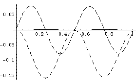
Here are the load objects. They are unchanged, except that GyroMoment uses the inertia option to explicitly specify the inertia properties. If this was not done, GyroMoment would pull the inertia properties from the body object that has previously had the X component filtered out. The model is now functionally equivalent to the previously defined model. The model can be integrated with SolveFree, after dropping constraints 2 and 4. Constraint 6 was previously dropped and is no longer part of the model. The model is integrated from T = 0 to 1. Here is a plot of the angular velocity components of the gimbal. It is identical to the response of the previous model, with only two bodies required to create it.
Out[35]= |  |
Undocumented Graphics Generation
|