CUDAFunctionLoad["src",fun,argtypes,blockdim]
文字列 src をコンパイルし,fun をCUDAFunctionとしてWolfram言語で使えるようにする.
CUDAFunctionLoad[File[srcfile],fun,argtypes,blockdim]
ソースコードファイル srcfile をコンパイルし,fun をCUDAFunctionとしてロードする.
CUDAFunctionLoad[File[libfile],fun,argtypes,blockdim]
以前コンパイルしたライブラリ libfile から,fun をCUDAFunctionとしてロードする.
CUDAFunctionLoad
CUDAFunctionLoad["src",fun,argtypes,blockdim]
文字列 src をコンパイルし,fun をCUDAFunctionとしてWolfram言語で使えるようにする.
CUDAFunctionLoad[File[srcfile],fun,argtypes,blockdim]
ソースコードファイル srcfile をコンパイルし,fun をCUDAFunctionとしてロードする.
CUDAFunctionLoad[File[libfile],fun,argtypes,blockdim]
以前コンパイルしたライブラリ libfile から,fun をCUDAFunctionとしてロードする.
詳細とオプション
- CUDALink パッケージがNeeds["CUDALink`"]でロードされていなければならない.
- 使用可能な引数と戻り型,対応するCUDA言語の型:
-
_Integer mint Wolfram言語整数 "Integer32" int 32ビット整数 "Integer64" long/long long 64ビット整数 _Real Real_t GPU実数型 "Double" double 機械倍精度数 "Float" float 機械浮動小数点数 {base, rank, io} CUDAMemory 指定の基底型,階数,入出力オプションのメモリ "Local" | "Shared" mint 局所または共有のメモリパラメータ {"Local" | "Shared", type} mint 局所または共有のメモリパラメータ - 指定{base, rank, io}において,有効なioは"Input","Output","InputOutput"である.
- 引数指定{base}は{base,_,"InputOutput"}に等しく,{base,rank}は{base,rank,"InputOutput"}に等しい.
- 階数は{base,_,io}または{base,io}を使うことで省略できる.
- 使用できる基底型:
-
_Integer _Real _Complex "Byte" "Bit16" "Integer32" "Byte[2]" "Bit16[2]" "Integer32[2]" "Byte[3]" "Bit16[3]" "Integer32[3]" "Byte[4]" "Bit16[4]" "Integer32[4]" "UnsignedByte" "UnsignedBit16" "UnsignedInteger" "UnsignedByte[2]" "UnsignedBit16[2]" "UnsignedInteger[2]" "UnsignedByte[3]" "UnsignedBit16[3]" "UnsignedInteger[3]" "UnsignedByte[4]" "UnsignedBit16[4]" "UnsignedInteger[4]" "Double" "Float" "Integer64" "Double[2]" "Float[2]" "Integer64[2]" "Double[3]" "Float[3]" "Integer64[3]" "Double[4]" "Float[4]" "Integer64[4]" - CUDAFunctionLoadは別の引数で複数回呼び出すこともできる.
- CUDAFunctionLoadでロードされた関数はWolfram言語カーネルと同じプロセスで実行される.
- CUDAFunctionLoadでロードされた関数はWolfram言語カーネルが終了するときにアンロードされる.
- ブロック次元には,1ブロックにつきいくつのスレッドを開始するかを表すリストまたは整数が使える.
- libfileがダイナミックライブラリなら,ダイナミックライブラリ関数 fun がロードされる.
- libfileにはCUDA PTX,CUDA CUBIN,ライブラリファイルが使える.
- ブロック次元の最大サイズはCUDAInformationの"Maximum Block Dimensions"特性で返される.
- 開始するときに,(CUDAFunctionへの追加の引数として)スレッド数が指定されてなければ,階数と次元が最も大きい要素の次元が選ばれる.画像については階数は2に設定される.
- 開始するときに,スレッド数がブロック時限の倍数でなければ,ブロック次元の倍数に切り上げられる.
- 以下のオプションが与えられる:
-
"CleanIntermediate" Automatic 一時ファイルを削除するかどうか "CompileOptions" {} NVCCコンパイラに直接渡すオプション "CompilerInstallation" Automatic CUDAツールキットがインストールされている場所 "CreateCUBIN" True コードをCUDAバイナリにコンパイルするかどうか "CreatePTX" False コードをCUDAバイトコードにコンパイルするかどうか "CUDAArchitecture" Automatic CUDAコードをコンパイルする目的アーキテクチャ "Defines" {} NVCCプリプロセッサに渡された定義 "Device" $CUDADevice 計算で使用するCUDAデバイス "IncludeDirectories" {} コンパイルに含むディレクトリ "ShellCommandFunction" None コンパイルで使用するシェルコマンドで呼び出す関数 "ShellOutputFunction" None コンパイルコマンドの実行によるシェル出力で呼び出す関数 "SystemDefines" Automatic NVCCプリプロセッサに渡されたシステム定義 "TargetDirectory" Automatic CUDAファイルが生成されるディレクトリ "TargetPrecision" Automatic 計算に使用する精度 "WorkingDirectory" Automatic 一時ファイルが生成されるディレクトリ "XCompilerInstallation" Automatic CコンパイラがインストールされていることをNVCCが探すディレクトリ
例題
すべて開く すべて閉じる例 (5)
Needs["CUDALink`"]code = "
__global__ void addTwo(mint * in, mint * out, mint length) {
int index = threadIdx.x + blockIdx.x*blockDim.x;
if (index < length)
out[index] = in[index] + 2;
}";cudaFun = CUDAFunctionLoad[code, "addTwo", {{_Integer, _, "Input"}, {_Integer, _, "Output"}, _Integer}, 256]listSize = 1000;入出力ベクトルを定義する.これらはWolfram言語の通常のリストで,CUDAカーネルコードのシグネチャで定義した型と同じである:
A = ConstantArray[1, {listSize}];
B = ConstantArray[1, {listSize}];res = cudaFun[A, B, listSize];Take[First@res,20]CUDAファイルがを渡すことができる.CUDA関数ファイルへのパスを表示する:
srcf = FileNameJoin[{$CUDALinkPath, "SupportFiles", "imageColorNegate.cu"}];colorNegate = CUDAFunctionLoad[File[srcf], "imageColorNegate", {{_Integer, _, "InputOutput"}, _Integer, _Integer, _Integer}, {16, 16}]{height, width, channels} = ImageDimensions[[image]]~Join~{ImageChannels[[image]]}colorNegate[[image], width, height, channels]CUDAFunctionを呼び出すときは追加の引数を与えることができる.引数は開始するスレッド数(またはグリッド次元とブロック次元の積)を表す.CUDA実装を含むソースファイルを取得する:
srcf = FileNameJoin[{$CUDALinkPath, "SupportFiles", "vecAdd.cu"}];vectorAdd = CUDAFunctionLoad[File[srcf], "vecAdd", {{_Integer, _, "Input"}, {_Integer, _, "Input"}, {_Integer, _, "Output"}, _Integer}, 16]32スレッドの関数を呼び出す.ベクトルの最初の32個の値の加算が計算される:
vectorAdd[Range[64], ConstantArray[2, 64], ConstantArray[0, 64], 256, 32]浮動小数点精度のサポートのために,ハードウェアと"TargetPrecision"に基づいてReal_tが定義されている:
code = "
__global__ void average(Real_t * in, Real_t * out, mint length) {
int index = threadIdx.x + blockIdx.x*blockDim.x;
if (index < length - 1)
out[index] = (in[index] + in[index+1]) / static_cast<Real_t>(2.0f);
else if (index == length - 1)
out[index] = in[index];
}";オプションを与えないと,"TargetPrecision"はデバイスで使用できる最高の浮動小数点精度を使用する.この場合は倍精度である:
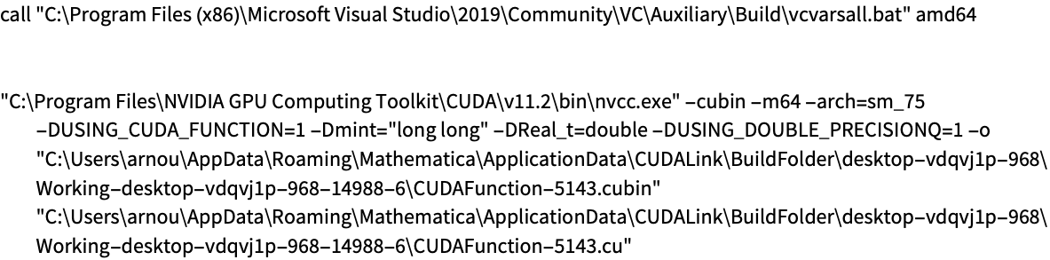
averageReal = CUDAFunctionLoad[code, "average", {{_Real, _, "Output"}, {_Real, _, "Input"}, _Integer}, {16, 16}, "ShellCommandFunction" -> Print]マクロReal_t=doubleとCUDALINK_USING_DOUBLE_PRECISIONQ=1がどのように定義されるかに注目されたい.検出を避けるために"Double"または"Single"オプションが渡せる.これは上のものと同じである:
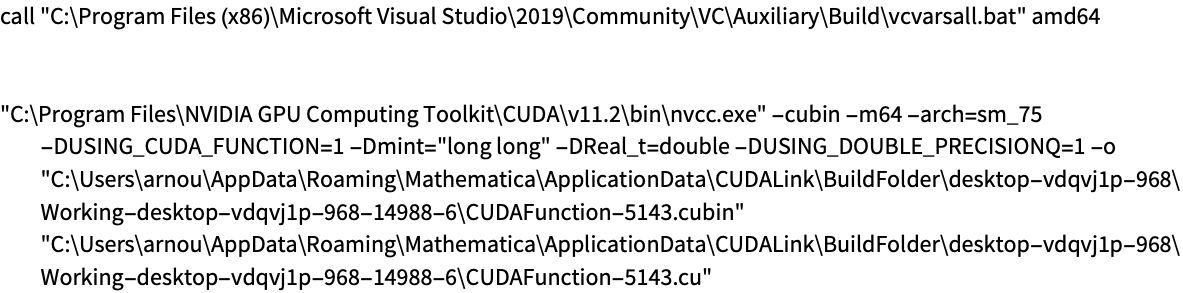
averageReal = CUDAFunctionLoad[code, "average", {{_Real, _, "Output"}, {_Real, _, "Input"}, _Integer}, {16, 16}, "ShellCommandFunction" -> Print, "TargetPrecision" -> "Double"]単精度の利用を強制するためには"TargetPrecision"に"Single"値を渡す:
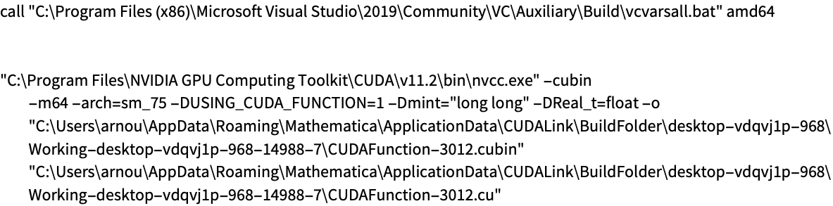
averageReal = CUDAFunctionLoad[code, "average", {{_Real, _, "Output"}, {_Real, _, "Input"}, _Integer}, {16, 16}, "ShellCommandFunction" -> Print, "TargetPrecision" -> "Single"]目的精度に基づいて型_Realが検出される.指定の型の使用を強制するために,型として"Float"または"Double"を渡す:
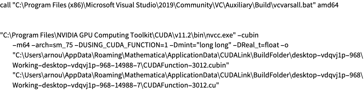
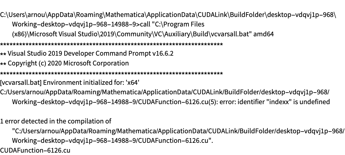
averageReal = CUDAFunctionLoad[code, "average", {{"Float", _, "Output"}, {"Float", _, "Input"}, _Integer}, {16, 16}, "ShellCommandFunction" -> Print, "TargetPrecision" -> "Single"]"ShellOutputFunction"を使ってコンパイルの失敗についての情報を得ることができる.ソースコードにシンタックスエラーがある:

code = "
__global__ void addTwo(mint * in, mint * out, mint length) {
int index = threadIdx.x + blockIdx.x*blockDim.x;
if (index < length)
out[index] = in[indexx] + 2;
}";cudaFun = CUDAFunctionLoad[code, "addTwo", {{_Integer, _, "Input"}, {_Integer, _, "Output"}, _Integer}, 256];
"ShellOutputFunction"->Printと設定すると,ビルドログが与えられる:

cudaFun = CUDAFunctionLoad[code, "addTwo", {{_Integer, _, "Input"}, {_Integer, _, "Output"}, _Integer}, 256, "ShellOutputFunction" -> Print];
スコープ (5)
CとCUDAファイルのロード (1)
CUDAFunctionLoadはコードのCの部分を無視する.これによりバイナリとしてそれ自体でコンパイルできるが,CUDAFunctionとしてもロードできるコードを書くことが可能となる.CUDAソースファイル(Cが混在したもの)をWolfram言語にロードする:
vecAdd = CUDAFunctionLoad[File[FileNameJoin[{$CUDALinkPath, "SupportFiles", "cudaDLL.cu"}]], "vecAdd", {{_Integer, _, "Input"}, {_Integer, _, "Output"}, _Integer}, 16, "IncludeDirectories" -> FileNameJoin[{$InstallationDirectory, "SystemFiles", "IncludeFiles", "C"}], "SystemDefines" -> {}]vecAdd[Range[100], Range[100], 100]共有または局所のメモリの指定 (2)
CUDAFunctionLoadはランタイムにおける関数の共有(局所)メモリサイズを指定することができる.次のコードは共有メモリを使って勾配の計算のための大域メモリを保管する:
code = "
__global__ void grad(mint * img, mint n) {
extern __shared__ mint smem[];
int tx = threadIdx.x;
int bx = blockIdx.x;
int dx = blockDim.x;
int index = tx + bx*dx;
#define S(txOffset) smem[txOffset + 1]
S(tx) = index < n ? img[index] : 0;
if (tx == 0) {
S(tx - 1) = index >= 0 ? img[index - 1] : 0;
} else if (tx == dx - 1) {
S(tx + 1) = index <= n-1 ? img[index + 1] : 0;
}
__syncthreads();
tx += 1;
if (index < n)
img[index] = (S(tx + 1) - S(tx-1))/2;
}";最後の引数が共有メモリのための"Shared"である入力引数を指定する.ブロックサイズは256に設定される:
fun = CUDAFunctionLoad[code, "grad", {{_Integer}, _Integer, "Shared"}, 256]n = Times@@ImageDimensions[[image]];関数を呼び出す.共有メモリサイズは(blockSize+2)*sizeof(mint)に設定され,開始するスレッド数は画像の平坦化された長さに設定される:
fun[[image], n, (256 + 2) * 8, n]共有メモリサイズを指定するよりよい方法は,型を使う方法である:
fun = CUDAFunctionLoad[code, "grad", {{_Integer}, _Integer, {"Shared", _Integer}}, 256]fun[[image], n, 256 + 2, n]テンプレート化された関数 (1)
テンプレート化された関数を呼び出すことができる.制約は,デバイス関数としてテンプレート化された関数のインスタンスを作成し,"UnmangleCode"をFalseに設定しなければならないということだけである.どのデバイス関数を呼び出すかを決めるディスパッチ関数を使って,テンプレート化された関数をコンパイルしてPTXバイトコードにする:
cmpf = CreateExecutable["
template <typename T>
__device__ void vecAdd_op(T * in, T * out, int index) {
out[index] += in[index];
}
extern \"C\" __global__ void vecAdd(int type, void * in, void * out, int width) {
int index = threadIdx.x + blockIdx.x*blockDim.x;
if (index < width) {
switch (type) {
case 0:
vecAdd_op<char>((char *) in, (char *) out, index);
break ;
case 1:
vecAdd_op<unsigned char>((unsigned char *) in, (unsigned char *) out, index);
break ;
case 2:
vecAdd_op<short>((short *) in, (short *) out, index);
break ;
case 3:
vecAdd_op<int>((int *) in, (int *) out, index);
break ;
}
}
}
", "templatedKernel", "Compiler" -> NVCCCompiler, "UnmangleCode" -> False, "CreatePTX" -> True, "TargetDirectory" -> $TemporaryDirectory];fun = CUDAFunctionLoad[File[cmpf], "vecAdd", {"Integer32", {"Integer32", _, "Input"}, {"Integer32", _, "Output"}, "Integer32"}, 16]関数を実行する.3は入力型が整数であることを指定するものである:
fun[3, Range[100], Range[100], 100]マクロを使用した汎用型 (1)
テンプレート化された関数はマクロを使って同じものが作れる.次のソースコードは未定義マクロとしてGeneric_tを持つ:
src = "__global__ void imageColorNegate(Generic_t * in, Generic_t * out, mint width, mint height, mint channels) {
mint ii;
mint xIndex = threadIdx.x + blockIdx.x*blockDim.x;
mint yIndex = threadIdx.y + blockIdx.y*blockDim.y;
mint index = channels*(xIndex + yIndex*width);
if (xIndex < width && yIndex < height) {
for (ii = 0; ii < channels; ii++)
out[index+ii] = 255 - in[index+ii];
}
}";intColorNegate = CUDAFunctionLoad[src, "imageColorNegate", {{_Integer, _, "Input"}, {_Integer, _, "Output"}, _Integer, _Integer, _Integer}, {16, 16}, "Defines" -> {"Generic_t" -> "mint"}]マクロGeneric_tをunsigned charに設定する:
intColorNegate = CUDAFunctionLoad[src, "imageColorNegate", {{"UnsignedByte", _, "Input"}, {"UnsignedByte", _, "Output"}, _Integer, _Integer, _Integer}, {16, 16}, "Defines" -> {"Generic_t" -> "\"unsigned char\""}]三次元ブロックサイズ (1)
三次元ブロックサイズもサポートされている.体積データを反転る:
src = "
__global__ void volumetricInvertKernel(mint * data, mint width, mint height, mint depth) {
unsigned int xpos = threadIdx.x + blockIdx.x*blockDim.x;
unsigned int ypos = threadIdx.y + blockIdx.y*blockDim.y;
unsigned int zpos = threadIdx.z;
unsigned int stride = blockDim.z;
unsigned int mempos = xpos + (ypos + zpos*height)*width;
unsigned int limit = depth - threadIdx.z;
for (mint ii = 0; ii < limit; ii += stride) {
data[mempos + height*width*ii] = 255 - data[mempos + height*width*ii];
}
}
";volumetricInverseFun = CUDAFunctionLoad[src, "volumetricInvertKernel", {{_Integer, _, "InputOutput"}, _Integer, _Integer, _Integer}, {8, 8, 4}]data = CUDAVolumetricDataRead[FileNameJoin[{$CUDALinkExampleDataPath, "stent8.raw"}], 512, 174];invertedData = First[volumetricInverseFun[data, 512, 512, 174, {512, 512}]];CUDAVolumetricRender[invertedData]アプリケーション (8)
パーリン(Perlin)ノイズ (1)
パーリンノイズは擬似テクスチャを生成するのに使われる一般的なアルゴリズムである.次はノイズ関数の教科書どおりの実装である:
srcf = FileNameJoin[{$CUDALinkPath, "SupportFiles", "noise.cu"}];Perlin = CUDAFunctionLoad[File[srcf], "classicPerlin", {{_Real, "Output"}, {"Integer32", "Input"}, _Real, _Real, _Real, _Real, _Real, _Real, "Integer32", "Integer32", "Integer32"}, {16, 16}];permutations = Join[(permutations = RandomSample[Range[0, 255]]), permutations];width = height = 256;
noise = CUDAMemoryAllocate[Real, {width, height}];amplitude = 0.5;
frequency = 1.0;
gain = 0.5;
lacunarity = 2.0;
scale = 20.0;
increment = 5.0;
depth = 0;パーリンノイズ関数を呼び出す.出力はCUDAMemoryハンドルである:
Perlin[noise, permutations, amplitude, frequency, gain, lacunarity, scale, increment, width, height, depth, {width, height}]ReliefImage[CUDAMemoryGet[noise]]結果にManipulateを使うと,パラメータを変化させて出力を見ることができる:
Manipulate[
ReliefImage[CUDAMemoryGet@First[Perlin[noise, permutations, amp, freq, gn, lac, scl, inc, width, height, depth]]],
{{amp, 0.5, "Amplitude"}, 0.01, 1.0},
{{freq, 1.0, "Frequency"}, 0.01, 3.0},
{{gn, 0.5, "Gain"}, 0.01, 3.0},
{{lac, 2.0, "Lacunarity"}, 0.01, 5.0},
{{scl, 20.0, "Scale"}, 0.01, 50.0},
{{inc, 1.0, "Increment"}, 0.1, 10.0}
]パーリンノイズで手続き型の地形を作成することができる.幅高さを定義し,地形のためのメモリを割り当てる:
width = height = 64;
noise = CUDAMemoryAllocate[Real, {width, height}];amplitude = 0.5;
frequency = 1.0;
gain = 0.5;
lacunarity = 2.0;
scale = 30.0;
increment = 5.0;
depth = 0;データを取り出し,標高マップを平坦にするのに画像処理関数を適用する:
data = CUDAMemoryGet[First[Perlin[noise, permutations, amplitude, frequency, gain, lacunarity, scale, increment, width, height, depth, {width, height}]]];
img = Image[data];
img = ColorCombine[{ColorCombine[{Lighter[img, 0.2], GaussianFilter[img, 2], Binarize[img, 0.2]}], GaussianFilter[Binarize[img], 10]}]ListPlot3D[data, Mesh -> None, Boxed -> False, InterpolationOrder -> 2, Axes -> False, RotationAction -> "Clip", PlotStyle -> Texture[img]]CUDAMemoryUnload[noise]ノイズのパラメータを変化させると,異なるパターンになる.木のテクスチャを作る:
width = height = 256;
noise = CUDAMemoryAllocate[Real, {width, height}];amplitude = 0.5;
frequency = 1.0;
gain = 0.5;
lacunarity = 0.5;
scale = 50.0;
increment = 5.0;
depth = 0;imageRecolor[img_, r_, g_, b_] := Image[{r * img, g * img, b * img}, Interleaving -> False]data = 20.0 * CUDAMemoryGet[First[Perlin[noise, permutations, amplitude, frequency, gain, lacunarity, scale, increment, width, height, depth, {width, height}]]];
imageRecolor[data - Map[IntegerPart, data, Infinity], 1.0, 0.4, 0.1]img = GaussianFilter[[image], 2];
data = ImageData[GaussianFilter[First[ColorSeparate[img]], 8]];
ListPlot3D[data, PlotStyle -> Texture[img], Mesh -> None, Axes -> None, Boxed -> False]もとのソースコードはより多くのノイズ関数を定義している.関数をロードする:
{Perlin, MultiFractal, Turbulence, RidgeMultifractal, MonoFractal} = CUDAFunctionLoad[File[srcf], #, {{_Real, _, "Output"}, {"Integer32", _, "Input"}, _Real, _Real, _Real, _Real, _Real, _Real, "Integer32", "Integer32", "Integer32"}, {16, 16}]& /@ {"classicPerlin", "multiFractal", "turbulence", "ridgeMultifractal", "monoFractal"};Manipulateを使って別のノイズ関数を示す:
Manipulate[
ReliefImage[CUDAMemoryGet@First[fun[noise, permutations, amp, freq, gn, lac, scl, inc, width, height, depth]]],
{{fun, Perlin, "Noise Function"}, {Perlin -> "Perlin", MultiFractal -> "MultiFractal", Turbulence -> "Turbulence", RidgeMultifractal -> "RidgeMultifractal", MonoFractal -> "MonoFractal"}},
{{amp, 0.5, "Amplitude"}, 0.01, 1.0},
{{freq, 1.0, "Frequency"}, 0.01, 3.0},
{{gn, 0.5, "Gain"}, 0.01, 3.0},
{{lac, 2.0, "Lacunarity"}, 0.01, 5.0},
{{scl, 20.0, "Scale"}, 0.01, 50.0},
{{inc, 1.0, "Increment"}, 0.1, 10.0}
]CUDAMemoryUnload[noise]ヒストグラムアルゴリズム (1)
ヒストグラムアルゴリズムは値によって要素を別々のビンのリストに分ける.次の例は0から255までの値を別々のビンに分けるヒストグラムを実装する:
srcf = FileNameJoin[{$CUDALinkPath, "SupportFiles", "histogram.cu"}];histogramKernel = CUDAFunctionLoad[File[srcf], "histogram256Kernel", {{"UnsignedInteger32", "Output"}, "UnsignedInteger32", {"UnsignedInteger32", "Input"}, "UnsignedInteger32"}, 192];
mergekernel = CUDAFunctionLoad[File[srcf], "mergeHistogram256Kernel", {{"UnsignedInteger32", _, "Output"}, {"UnsignedInteger32", _, "Input"}, "UnsignedInteger32"}, 256];サンプルデータを取得する.この場合は画像が選ばれ,ImageDataを平坦化する:
data = Flatten[ImageData[[image], "Byte"]];
dataLength = Length[data];アルゴリズムには中間ヒストグラムに使われる一時データが必要である:
partialHistograms = CUDAMemoryAllocate["UnsignedInteger32", 256 * 240];
histogram = CUDAMemoryLoad[ConstantArray[0, 256], "UnsignedInteger32"];
partialHistogramCount = 240;部分ヒストグラムを計算し,それを前に生成した中間リストに置く:
histogramKernel[partialHistograms, 1, data, dataLength, 240 * 192];mergekernel[histogram, partialHistograms, partialHistogramCount, 256 * 256];outputHistogram = CUDAMemoryGet[histogram];一時メモリをアンロードする.これを行わないと,メモリリークが起こる:
CUDAMemoryUnload[partialHistograms, histogram]ListLinePlot[outputHistogram, InterpolationOrder -> 0]プレフィックス和アルゴリズム (1)
Needs["CUDALink`"]走査,つまりプレフィックス和はFoldListに似ており,さまざまな状況で使える非常に便利なプリミティブである.CUDAの実装は以下にある:
srcf = FileNameJoin[{$CUDALinkPath, "SupportFiles", "scan_kernel.cu"}];scanExclusiveShared = CUDAFunctionLoad[File[srcf], "scanExclusiveShared", {{"Integer32[4]", _, "Output"}, {"Integer32[4]", _, "Input"}, "Integer32", "Integer32", "Integer32"}, 256];
scanExclusiveShared2 = CUDAFunctionLoad[File[srcf], "scanExclusiveShared2", {{"Integer32", "InputOutput"}, {"Integer32", "Output"}, {"Integer32", "Input"}, "Integer32", "Integer32", "Integer32", "Integer32"}, 256];
uniformUpdate = CUDAFunctionLoad[File[srcf], "uniformUpdate", {{"Integer32[4]", "InputOutput"}, {"Integer32[4]", "InputOutput"}, "Integer32", "Integer32"}, 256];data = RandomInteger[10, 128];dest = CUDAMemoryAllocate[Integer, 128];blockDim = 256;
gridDim = blockDim * Ceiling[Length[data] / (4 * blockDim)];buffer = CUDAMemoryAllocate[Integer, 1 + (gridDim / blockDim)];scanExclusiveShared[dest, data, 4 * blockDim, 1, 0, gridDim];
scanExclusiveShared2[buffer, dest, data, 1 + (gridDim / blockDim), 1 + (gridDim / blockDim), 1, 0];
uniformUpdate[dest, buffer, 1, 0];CUDAMemoryGet[dest]結果はFoldListのものと一致する:
FoldList[Plus, 0, data]CUDAMemory要素の割当てを解放する:
CUDAMemoryUnload[dest, buffer]リダクション (1)
リダクションカーネルは指定のバイナリ操作によるリストのリダクションという意味で,Wolfram言語のFoldに似ている.操作が計算で前の要素を維持するのに対し,リダクションはそれを削除する.
リダクションCUDAFunctionをロードする:
reduce = CUDAFunctionLoad[File[FileNameJoin[{$CUDALinkPath, "SupportFiles", "reduce.cu"}]], "reduce", {{_Integer, 1, "Input"}, {_Integer, 1, "Output"}, "Integer32"}, {256}, "Defines" -> {"T1" -> "mint", "BLOCK_SIZE" -> 256, "nIsPow2" -> 0}]in = ConstantArray[1, 131072];
out = CUDAMemoryAllocate[Integer, 256];reduce[in, out, 131072]各ブロックはリストの512要素のリダクションを行う.つまり,512要素より大きいリストのリダクションには複数回の呼出しが必要となる.次のリストは小さく,ループが必要ない.前のステップから出力メモリを取得し,outのメモリをinに割当て,outを解放する:
in = CUDAMemoryGet[out];
CUDAMemoryUnload[out];out = CUDAMemoryAllocate[Integer, 1];reduce[in, out, 256]CUDAMemoryGet[out]
CUDAMemoryUnload[out];Total[in]RGBからHSBへの変換 (1)
次の例はRGB色空間からHSBへの色の変換を実装する.CUDAによる実装は以下のファイルにある:
srcf = FileNameJoin[{$CUDALinkPath, "SupportFiles", "colorConvert.cu"}]RGB2HSB = CUDAFunctionLoad[File[srcf], "rgb2hsb", {{_Real, 3, "Input"}, {_Real, 3, "Output"}, _Integer, _Integer, _Integer, _Integer}, {16, 16}]img = [image];
{height, width} = ImageDimensions[img];
channels = ImageChannels[img];
pitch = channels * width;output = CUDAMemoryAllocate[Real, {height, width, channels}]RGB2HSB[img, output, width, height, channels, pitch, {width, height}]デフォルトでは,ImageはRGB色空間のデータを見る.結果は間違った出力となる:
Image[CUDAMemoryGet[output]]適切な出力を得るためにColorSpace -> "HSB"を使う:
Image[CUDAMemoryGet[output], ColorSpace -> "HSB"]シーザー(Caesar)暗号 (1)
次のコードはシーザー暗号を実装する.シーザー暗号はテキストの各文字に3を足す簡単な暗号法である.以下がCUDAの実装である:
code = "
__global__ void caesarCipher(char * text, mint length) {
mint index = threadIdx.x + blockIdx.x*blockDim.x;
if (index < length) {
char c = text[index];
if ((c >= 'a' && c <= 'z') ||
(c >= 'A' && c <= 'Z')) {
c += 3;
if (c > 'z' || (c < 'a' && c > 'Z'))
c -= 26;
}
text[index] = c;
}
}";例に使うテキストをロードする.この場合はアメリカ独立宣言書がロードされる:
DOI = ToCharacterCode[ExampleData[{"Text","DeclarationOfIndependence"}]];CaesarCipher = CUDAFunctionLoad[code, "caesarCipher", {{"Byte"}, _Integer}, 256]StringTake[FromCharacterCode[First@CaesarCipher[DOI, Length[DOI]]], 100]移動平均 (1)
src = "
__global__ void movingAverage(mint * in, mint * out, mint n) {
__shared__ mint smem[BLOCK_DIM + 1];
mint tx = threadIdx.x;
mint bx = blockIdx.x;
mint dx = blockDim.x;
mint index = tx + bx*dx;
if (index < n)
smem[tx] = in[index];
else
smem[tx] = in[n - 1];
if (tx == dx-1) {
if (index - 1 < n) {
smem[bx] = in[index+1];
} else {
smem[bx] = in[n-1];
}
}
__syncthreads();
if (index < n)
out[index] = (smem[tx] + smem[tx+1])/2;
}
";マクロ"BLOCK_DIM"を256として定義するCUDAFunctionをロードする:
movingAverage = CUDAFunctionLoad[src, "movingAverage", {{_Integer, "Input"}, {_Integer, "Output"}, _Integer}, 256, "Defines" -> {"BLOCK_DIM" -> 256}]len = 100;
input = RandomInteger[100, len];
output = CUDAMemoryAllocate[Integer, len];CUDAFunctionを呼び出す:
movingAverage[input, output, len]CUDAMemoryGet[output]CUDAMemoryUnload[output]ブラック–ショールズ(Black–Scholes)方程式 (1)
ブラック–ショールズ方程式はよく金融の計算で使われる.CUDALink にはCUDAFinancialDerivativeがあり,これは金融オプションの計算ができる.これがどのように書かれているかを例示するために,簡単なバージョンを実装する:
srcf = FileNameJoin[{$CUDALinkPath, "SupportFiles", "blackScholes_simple.cu"}]CUDAFunctionをロードする._Realが"Float"として解釈されるように"TargetPrecision"を"Single"に設定する:
BlackScholes = CUDAFunctionLoad[File[srcf], "BlackScholes", {{_Real, _, "Output"}, {_Real, _, "Output"}, {_Real, _, "Input"}, {_Real, _, "Input"}, {_Real, _, "Input"}, _Real, _Real, _Integer}, 128, "TargetPrecision" -> "Single"]numberOfOptions = 64;
call = CUDAMemoryAllocate["Float", numberOfOptions];
put = CUDAMemoryAllocate["Float", numberOfOptions];
currentPrices = RandomReal[{25.0, 35.0}, numberOfOptions];
strikePrices = RandomReal[{20.0, 40.0}, numberOfOptions];
strikeTimes = RandomReal[{0.1, 10.0}, numberOfOptions];
riskFree = 0.02;
volatility = 0.30;BlackScholes[call, put, currentPrices, strikePrices, strikeTimes, riskFree, volatility, numberOfOptions, numberOfOptions]CUDAMemoryGet[call]CUDAMemoryUnload[call, put]考えられる問題 (4)
最大ブロック次元がCUDAInformationによって返される:
CUDAInformation[$CUDADevice, "Maximum Block Dimensions"]関数呼び出しにおけるエラーは CUDALink を不安定な状態にすることがある.これはユーザが任意のカーネルを書くことができるようにすることの副作用である.カーネルコード中の無限ループやバッファのオーバーフロー等は CUDALink とビデオドライバの両方を不安定な状態にすることがある.
これは極端な場合,ディスプレイドライバをクラッシュさせることがあるが,通常はCUDAコードのその後の評価で無効な結果が返されるだけである.
コンパイル済みカーネルの型は一致しなければならない.浮動小数点数として定義されたReal_tのカーネルは,"TargetPrecision"が"Double" に設定されているときに使うと不正な結果を返す.
"UnmangleCode"がTrueに設定されているときは,C++構文のエキスポートはサポートされていない.
インタラクティブな例題 (4)
コンウェイ(Conway)のライフゲーム (1)
コンウェイのライフゲームは周りの状態に基づいて進化するセルオートマトンである.CUDALink 関数をロードする:
gol = CUDAFunctionLoad[File[FileNameJoin[{$CUDALinkPath, "SupportFiles", "gol.cu"}]], "gol_kernel", {{_Integer, _, "Input"}, {_Integer, _, "Output"}, _Integer, _Integer}, {16, 16}]初期化のためにランダムに初期化する必要があるが,極端に少ない初期状態にするとすべてのセルが死んでしまうので避けなければならない:
initialState = ConstantArray[0, {512, 512}];
Do[
With[{x = RandomInteger[{1, 512}], y = RandomInteger[{1, 512}], n = RandomInteger[3]},
initialState[[x, y]] = 1;
MapThread[(initialState[[Mod[x + #1, 512] + 1, Mod[y + #2, 512] + 1]] = 1)&, {Range[-1, 1][[ ;; n]], Range[-1, 1][[ ;; n]]}]
],
{10000}
];
outputState = ConstantArray[0, {512, 512}];Dynamic[
Refresh[
initialState = First[gol[initialState, outputState, 512, 512]];ArrayPlot[initialState, ImageSize -> Medium],
UpdateInterval -> 1 / 60
]
]DynamicとImageを使って関数を表示する.少し速いことに注目されたい:
Dynamic[
Refresh[
initialState = First[gol[initialState, outputState, 512, 512]];Image[initialState, "Bit"],
UpdateInterval -> 0
]
]CUDAMemoryを使うと,描画速度を上げることができる:
initialMem = CUDAMemoryLoad[initialState];
outputMem = CUDAMemoryLoad[outputState];
Dynamic[
Refresh[
gol[initialMem, outputMem, 512, 512];
gol[outputMem, initialMem, 512, 512];
Image[CUDAMemoryGet[initialMem], "Bit"],
UpdateInterval -> 0
]
]ボールの跳ね (1)
次の関数はCUDAFunctionをロードし,BallBounceEffect関数を呼び出す:次の物理的シミュレーションでは,CUDAFunctionを使って計算を行い,残りをWolfram言語に任せる方法を示す.
BallBouncePattern[] :=
Module[{code, bb, BlockDim},
code = "
#include <math.h>
__global__ void bb(Real_t* v, Real_t* z, Real_t* r, mint *state, Real_t acc, mint size, mint seq) {
mint ix = threadIdx.x + blockIdx.x*blockDim.x;
mint iy = threadIdx.y + blockIdx.y*blockDim.y;
mint i=ix*size+iy;
if(ix < size && iy < size &&
sqrt((float)( (ix-size/2)*(ix-size/2)+(iy-size/2)*(iy-size/2) ) ) >=(float)seq ) {
if(v[i]<0) {
v[i]=0;
state[i]=1;
}
if(z[i]<0) {
z[i]=0;
state[i]=-1;
}
v[i]+=state[i]*acc*r[i]/.25;
z[i]-=state[i]*v[i];
}
}";
BlockDim = {8, 8};
bb = CUDAFunctionLoad[code, "bb", {{"Float"}, {"Float"}, {"Float", _, "Input"}, {_Integer}, _Real, _Integer, _Integer}, BlockDim, "TargetPrecision" -> "Single"];
Mouseover[Graphics[{LightGray, Circle[], Inset[Style["Bring Mouse Here", Bold, Blue]]}], BallBounceEffect[bb]
]
]BallBounceEffect[bb1_] :=
Module[{tsize, fsize, z, r1, r, v, acc, device, state, za, ra, va, sa, code, BlockDim, GridDim, res, res1, res2, vc, s},
tsize = 101;
fsize = 80;
z = Table[fsize - 2 + RandomReal[2], {i, tsize * tsize}];
r = Table[.25, {i, tsize * tsize}];
v = ConstantArray[0.0, tsize * tsize];
acc = 0.2;
s = Ceiling[tsize / Sqrt[2]];
device = Automatic;
state = ConstantArray[1, tsize * tsize];
vc = Map[ColorData["BrightBands"], Range[0, 1, 1 / (tsize ^ 2 - 1)]] //. RGBColor -> List;
Graphics3D[{AbsolutePointSize[0],
Point[Dynamic[Refresh[
{v, z, state} = bb1[v, z, r, state, acc, tsize, s--, {tsize, tsize}];
Flatten[Table[{i, j, z[[(i - 1) * tsize + j]]}, {i, tsize}, {j, tsize}], 1], UpdateInterval -> 0]], VertexColors -> vc], Sphere[{tsize / 2, tsize / 2, -10}, .05], Sphere[{tsize / 2, tsize / 2, fsize}, .05],
{Black, Polygon[{{tsize, 0, 0}, {tsize, tsize, 0}, {0, tsize, 0}, {0, 0, 0}}]}
}, Boxed -> False]
]BallBouncePattern[]ジュリア(Julia)集合 (1)
ジュリア集合はマンデルブロ(Mandelbrot)集合を一般化したものである.CUDAカーネルを実装する:
code = "
__global__ void julia_kernel(Real_t * set, mint width, mint height, Real_t cx, Real_t cy) {
mint xIndex = threadIdx.x + blockIdx.x*blockDim.x;
mint yIndex = threadIdx.y + blockIdx.y*blockDim.y;
mint ii;
Real_t x = ZOOM_LEVEL*(width/2 - xIndex);
Real_t y = ZOOM_LEVEL*(height/2 - yIndex);
Real_t tmp;
Real_t c;
if (xIndex < width && yIndex < height) {
for (ii = 0; ii < MAX_ITERATIONS && x*x + y*y < BAILOUT; ii++) {
tmp = x*x - y*y + cx;
y = 2*x*y + cy;
x = tmp;
}
c = logf(static_cast<Real_t>(0.1) + sqrtf(x*x + y*y));
set[xIndex + yIndex*width] = c;
}
}
";幅と高さを設定する.集合は計算されるので,メモリを設定する必要はない.メモリ割当てのみが必要である:
{width, height} = {512, 512};
jset = CUDAMemoryAllocate[Real, {height, width}];CUDAFunctionをロードする.コンパイラがコードを最適化するのにループを解くようなことを行うマクロが使用される:
JuliaCalculate = CUDAFunctionLoad[code, "julia_kernel", {{_Real, _, "Output"}, _Integer, _Integer, _Real, _Real}, {16, 16}, "Defines" -> {"MAX_ITERATIONS" -> 10, "ZOOM_LEVEL" -> "0.0050", "BAILOUT" -> "4.0"}];集合を計算し,ReliefImageを使ってそれを見る:
JuliaCalculate[jset, width, height, 0.4, 0.2, {width, height}];
ReliefImage[Reverse@CUDAMemoryGet[jset], ImageSize -> 256]ManipulateとReliefPlotを使って,ユーザが
の値を調整することができるインターフェースを作る:
Manipulate[
JuliaCalculate[jset, width, height, c[[1]], c[[2]], {width, height}];
ReliefPlot[Reverse@CUDAMemoryGet[jset], ColorFunction -> "Rainbow", DataRange -> {{-2.0, 2.0}, {-2.0, 2.0}}, ImageSize -> 256],
{{c, {0, 1}}, {-2, -2}, {2, 2}, Locator}]ReliefPlotをImageに変えて可視化をより速くすることもできる:
Manipulate[JuliaCalculate[jset, width, height, c, d, {width, height}]; Image[CUDAMemoryGet[jset], ImageSize -> 256], {{c, 0.0}, -2.0, 2.0, Slider}, {{d, 0.0}, -2.0, 2.0, Slider}]マンデルブロ集合 (1)
マンデルブロ集合は
で定義される.次のコードは
(
はユーザ定義のパラメータ)という形式の集合を使って,カーネルファイルに独自のタイプをどのように定義するかを示す.カーネルは以下に定義されている:
srcf = FileNameJoin[{$CUDALinkPath, "SupportFiles", "mandelmorph.cu"}]{width, height} = {1024, 1024};出力集合のメモリはCUDAMemoryAllocateを使って割り当てる:
mset = CUDAMemoryAllocate["UnsignedByte", {height, width, 3}];MandelbrotMorph = CUDAFunctionLoad[File[srcf], "mandelbrot_kernel", {{"UnsignedByte", _, "Output"}, "Float", "Float", _Integer, _Integer}, {16, 16}, "Defines" -> {"MAX_ITERATIONS" -> 300, "BAILOUT" -> "8.0"}, "UnmangleCode" -> False]MandelbrotMorph[mset, 2.0, 0.0023, width, height];
Image[CUDAMemoryGet[mset], "Byte"]Manipulate[
MandelbrotMorph[mset, pow, 0.0023, width, height];
Image[CUDAMemoryGet[mset], "Byte", ImageSize -> 256], {{pow, 2.0, "Z Power"}, 1.0, 10.0}]width = height = 256;
mset = CUDAMemoryAllocate["UnsignedByte", {height, width, 3}];GraphicsGrid[Partition[imgs = (MandelbrotMorph[mset, #, 0.015, 256, 256];Image[CUDAMemoryGet[mset], "Byte"])& /@ Range[3.0, 5.0, 0.01], 20]]Style[Graphics3D[{Texture[ImageData /@ imgs], Black, Opacity[0.025], EdgeForm[None], Polygon[Table[{{-10, -10, z}, {10, -10, z}, {10, 10, z}, {-10, 10, z}}, {z, 0, 20, .1}], VertexTextureCoordinates -> Table[{{0, 0, s}, {0, 1, s}, {1, 1, s}, {1, 0, s}}, {s, 0, 1, .005}]]}, Background -> Black, Boxed -> False], "HardwareDepthBuffer" -> False]おもしろい例題 (4)
SymbolicCコードの生成 (1)
CUDALink の記号機能を使うと,Wolfram言語式を使ってCUDAコードを書き,それをCUDAコードに変換することができる.次の例では,記号コードを使って簡単な1D離散Haarウェーブレット変換を実装する:
symbolicCode = SymbolicCUDAFunction["dwtStep", {{CPointerType["mint"], "in"}, {CPointerType["mint"], "out"}, {"mint", "length"}, {"mint", "maxstage"}},
CBlock[{
SymbolicCUDADeclareIndexBlock[1],
CProgram["
while ( maxstage >=1){
if (index < length/2) {
mint left = in[2*index];
mint right = 2*index < length ? in[(2*index)+1] : 0;
out[index] = (left+right);
in[index] = out[index];
out[index+(length/2)] = (left-right);
}
maxstage = maxstage - 1;
length = length/2;
}
"]}]];記号コードはSymbolicCのToCCodeStringを使ってCUDAコードに変換できる:
ToCCodeString[symbolicCode]コードはCUDAFunctionLoadを使ってロードできる:
dwt = CUDAFunctionLoad[ToCCodeString[symbolicCode], "dwtStep", {{_Integer, _, "Input"}, {_Integer, _, "Output"}, _Integer, _Integer}, 256]A = ConstantArray[1, 10];
B = CUDAMemoryAllocate[Integer, Length[A]];
lengthA = Length[A];
maxStage = 1;maxStage=1としてCUDAFunctionを呼び出す:
dwt[A, B, lengthA, maxStage]結果のCUDAMemoryを取得する:
CUDAMemoryGet[B]記号コード生成の面白いのは,シンタックスツリーを操作することができるという点である.この例では,関数引数をCPointerType["int"]からCPointerType["float"]に変更する:
symbolicCode //. CPointerType["mint"] -> CPointerType["float"]ToCCodeString[%]コード生成のもう一つの面白い点は,CUDA記号関数はOpenCl記号関数のミラーとなっている点である.したがって上記記号コードのCUDA記号関数を変更するだけでOpdnCLコードを生成することができる:
Needs["OpenCLLink`"]OpenCLの1D離散Harrウェーブレット変換を実装する:
SymbolicOpenCLFunction["dwtStep", {{CPointerType["mint"], "in"}, {CPointerType["mint"], "out"}, {"mint", "length"}, {"mint", "maxstage"}},
CBlock[{
SymbolicOpenCLDeclareIndexBlock[1],
CProgram["
while ( maxstage >=1){
if (index < length/2) {
mint left = in[2*index];
mint right = 2*index < length ? in[(2*index)+1] : 0;
out[index] = (left+right);
in[index] = out[index];
out[index+(length/2)] = (left-right);
}
maxstage = maxstage - 1;
length = length/2;}
}
"]}]]//ToCCodeStringこの変換ではSymbolicCUDAFunctionをSymbolicOpenCLFunction,SymbolicCUDADeclareIndexBlockをSymbolicOpenCLDeclareIndexBlockという2語だけの変更が行われた.
マンデルブロ集合 (1)
code = "
__global__ void mandelbrot_kernel(unsigned char * set, mint width, mint height) {
mint xIndex = threadIdx.x + blockIdx.x*blockDim.x;
mint yIndex = threadIdx.y + blockIdx.y*blockDim.y;
mint ii;
Real_t x0 = ZOOM_LEVEL*(width/3 - xIndex);
Real_t y0 = ZOOM_LEVEL*(height/2 - yIndex);
Real_t tmp, x = 0, y = 0;
Real_t c;
if (xIndex < width && yIndex < height) {
for (ii = 0; (x*x+y*y <= BAILOUT) && (ii < MAX_ITERATIONS); ii++) {
tmp = x*x - y*y +x0;
y = 2*x*y + y0;
x = tmp;
}
c = ii - log(log(sqrt(x*x + y*y)))/log(2.0);
if (ii == MAX_ITERATIONS) {
set[3*(xIndex + yIndex*width)] = 0;
set[3*(xIndex + yIndex*width) + 1] = 0;
set[3*(xIndex + yIndex*width) + 2] = 0;
} else {
set[3*(xIndex + yIndex*width)] = ii*c/3 + 50;
set[3*(xIndex + yIndex*width) + 1] = ii*c;
set[3*(xIndex + yIndex*width) + 2] = ii*c + 30;
}
}
}
";{width, height} = {2048, 1024};mset = CUDAMemoryAllocate["UnsignedByte", {height, width, 3}];MandelbrotCalculate = CUDAFunctionLoad[code, "mandelbrot_kernel", {{"UnsignedByte", _, "Output"}, _Integer, _Integer}, {16, 16}, "Defines" -> {"MAX_ITERATIONS" -> 1000, "ZOOM_LEVEL" -> "0.0017", "BAILOUT" -> "8.0"}]MandelbrotCalculate[mset, width, height, {width, height}]Image[CUDAMemoryGet[mset], "Byte"]ルール30のセルオートマトン (1)
ルール30のセルオートマトンでは,隣の行は前のものに依存するため,列数が非常に大きくなるまではCUDAを使う利点はあまりない.それでも簡単なルール30のセルオートマトンをCUDA関数として書くことができる:
rule30 = CUDAFunctionLoad[File[FileNameJoin[{$CUDALinkPath, "SupportFiles", "rule30_ca.cu"}]], "rule30ca_kernel", {{_Integer, _, "Input"}, {_Integer, _, "Output"}, _Integer}, 256]prevRow = ConstantArray[0, 256];
prevRow[[128]] = 1;
nextRow = ConstantArray[0, 256];
ca = {prevRow};Do[
res = rule30[prevRow, nextRow, 256];
prevRow = First[res];
AppendTo[ca, prevRow],
{128}
];ArrayPlotを使って結果をプロットする:
ArrayPlot[ca]マンデルバルブ集合 (1)
次の実装は3Dにおけるマンデルブロ集合に類似した三次元マンデルブロ(マンデルバルブ)を実装する.三次元数は複素指数の極を

というように三次元空間座標に拡張する.加算は単純にベクトルの加算である.マンデルバルブパラメータ(幅,高さ,カメラ位置,光源位置)を指定する:
width = 640;
height = 480;
iconfig = {width, height, 1, 0, 1, 6};
config = {0.001, 0.0, 0.0, 0.0, 8.0, 15.0, 10.0, 5.0};
camera = {{2.0, 2.0, 2.0}, {0.0, 0.0, 0.0}};
AppendTo[camera, Normalize[camera[[2]] - camera[[1]]]];
AppendTo[camera, 0.75 * Normalize[Cross[camera[[3]], {0.0, 1.0, 0.0}]]];
AppendTo[camera, 0.75 * Normalize[Cross[camera[[4]], camera[[3]]]]];
config = Join[{config, Flatten[camera]}];pixelsMem = CUDAMemoryAllocate["Float", {height, width, 3}]srcf = FileNameJoin[{$CUDALinkPath, "SupportFiles", "mandelbulb.cu"}]CUDAFunctionを実装する:
mandelbulb = CUDAFunctionLoad[File[srcf], "MandelbulbGPU", {{"Float", _, "Output"}, {"Float", _, "Input"}, {"Integer32", _, "Input"}, "Integer32", "Float", "Float"}, {16}, "UnmangleCode" -> False]CUDAFunctionを実行する:
mandelbulb[pixelsMem, Flatten[config], iconfig, 0, 0.0, 0.0, {width * height * 3}];CUDAMemoryをWolfram言語に取り込む:
pixels = CUDAMemoryGet[pixelsMem];Image[pixels]結果をManipulateに置くことができる:
srcf = FileNameJoin[{$CUDALinkPath, "SupportFiles", "mandelbulb.cu"}];mandelbulb = CUDAFunctionLoad[File[srcf], "MandelbulbGPU", {{"Float", _, "Output"}, {"Float", _, "Input"}, {"Integer32", _, "Input"}, "Integer32", "Float", "Float"}, {16}, "UnmangleCode" -> False]width = 640;
height = 480;
pixelsMem = CUDAMemoryAllocate["Float", {height, width, 3}];Manipulate[
iconfig = { width, height, 1, 0, 1, 6};
config = {0.001, 0.0, 0.0, 0.0, 8.0, 15.0, 10.0, 5.0};
camera = {{cameraPosX, cameraPosY, cameraPosZ}, {cameraDirectionX, cameraDirectionY, cameraDirectionZ}};
AppendTo[camera, Normalize[camera[[2]] - camera[[1]]]];
AppendTo[camera, 0.75 * Normalize[Cross[camera[[3]], {0.0, 1.0, 0.0}]]];
AppendTo[camera, 0.75 * Normalize[Cross[camera[[4]], camera[[3]]]]];
config = 1.0 * Join[{config, Flatten[camera]}];
mandelbulb[pixelsMem, Flatten[config], iconfig, 0, 0.0, 0.0, {width * height}];
pixels = CUDAMemoryGet[pixelsMem];
Image[pixels], {{cameraPosX, 2.0, "Camera X Position"}, 0.0, 4.0}, {{cameraPosY, 2.0, "Camera Y Position"}, 0.0, 4.0}, {{cameraPosZ, 2.0, "Camera Z Position"}, 0.0, 4.0}, {{cameraDirectionX, 0.0, "Camera X Direction"}, 0.0, 1.0}, {{cameraDirectionY, 0.0, "Camera Y Direction"}, 0.0, 1.0}, {{cameraDirectionZ, 0.0, "Camera Z Direction"}, 0.0, 1.0}, SynchronousUpdating -> False]テクニカルノート
-
▪
- CUDALink ユーザガイド ▪
- CUDAプログラミング ▪
- 適用例
関連するガイド
-
▪
- CUDALink
テキスト
Wolfram Research (2010), CUDAFunctionLoad, Wolfram言語関数, https://reference.wolfram.com/language/CUDALink/ref/CUDAFunctionLoad.html.
CMS
Wolfram Language. 2010. "CUDAFunctionLoad." Wolfram Language & System Documentation Center. Wolfram Research. https://reference.wolfram.com/language/CUDALink/ref/CUDAFunctionLoad.html.
APA
Wolfram Language. (2010). CUDAFunctionLoad. Wolfram Language & System Documentation Center. Retrieved from https://reference.wolfram.com/language/CUDALink/ref/CUDAFunctionLoad.html
BibTeX
@misc{reference.wolfram_2026_cudafunctionload, author="Wolfram Research", title="{CUDAFunctionLoad}", year="2010", howpublished="\url{https://reference.wolfram.com/language/CUDALink/ref/CUDAFunctionLoad.html}", note=[Accessed: 13-August-2026]}
BibLaTeX
@online{reference.wolfram_2026_cudafunctionload, organization={Wolfram Research}, title={CUDAFunctionLoad}, year={2010}, url={https://reference.wolfram.com/language/CUDALink/ref/CUDAFunctionLoad.html}, note=[Accessed: 13-August-2026]}