Electric Motor Noise Analysis

Introduction	Model without Sound Barrier
Pressure Acoustics Model	Model with a Sound Barrier
Domain	Nomenclature
Boundary Conditions

Introduction

Noise analysis is an important phase when designing electrical motor driven systems. As a motor rotates, the harmonic electromagnetic forces between the rotor and stator continuously deform the outer casing of the motor. These periodic deformations lead to structural vibrations, which excite pressure waves to the surroundings as a noise.

The following model simulates the acoustic wave radiation from a motor spinning at , and . First, we will compute the sound pressure level (SPL) in the surrounding field to quantify the noise generation. In a subsequent step a sound barrier will be placed in the domain to reduce noise in a specific direction. The resulting sound pressure field will then be compared to the free-space case to measure the effectiveness of the sound barrier.

A related example that simulates the magnetic potential and the magnetic flux field within the electric motor is presented in a separate notebook entitled "Solving Partial Differential Equations with Finite Elements".

The symbols and corresponding units used throughout this tutorial are summarized in the Nomenclature section.

As a theoretical background for acoustics, please refer to the information provided in "Acoustics in the Frequency Domain".

Load the finite element package.

Pressure Acoustics Model

To model the time-harmonic deformation of the electrical motor, the acoustic model is built in the frequency domain. The propagation of harmonic sound waves can be described by the source-free Helmholtz partial differential equation (PDE) (1):

Define the variables and select the parameters for a frequency domain acoustics model.

Air is used as the sound medium.

Define material parameters for the acoustics PDE.

Domain

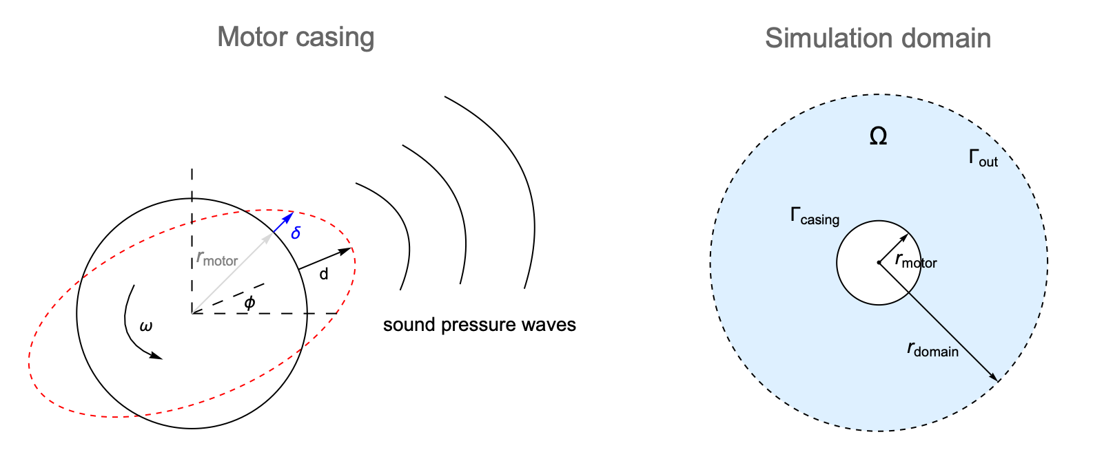
Consider the motor spinning at an angular frequency , the magnetic forces between the rotor and stator will continuously deform the outer casing of the motor. This periodic deformation can be approximately described by the cosine function:

In this model the maximum radial deformation of the motor is set as . Note that is assumed to be independent of the motor speed . This is a reasonable approximation since the eigenfrequencies of the motor are packed so closely in the high frequency range, and have little impact on the structural deformation.

More information on eigenfrequency analysis can be found in the "Acoustics in the Frequency Domain" tutorial.

The polar angle is defined as the angle measured from the -axis to the point on the motor casing:

To analyze the noise propagation in the surrounding area, the simulation domain is defined as a circular region enclosing the electric motor. The radius of the motor and the domain are and , respectively. The far-field boundary and the motor casing are symbolized as and , respectively.

Set the geometry parameters and the 2D domain

In acoustics simulations the wavelength of a sound wave needs to be resolved by a sufficiently fine mesh in order to get an accurate numerical solution. Here we set the max edge length to 12 nodes per , which means that there will be at least twelve elements per wavelength in each direction of the wave propagation.

More information on mesh size requirements for acoustic models can be found in the "Acoustics in the Frequency Domain" tutorial.

Compute the minimum wavelength

based on the maximum motor speed

Discretize the domain

Boundary Conditions

There are two types of the boundary conditions involved in this example. On the motor casing a normal velocity boundary condition is used to model the structural vibration.

Recall that the deformation of the casing is approximately described by a cosine function as:

For analytical convenience, equation (2) is converted into the complex exponential representation (CER):

The corresponding vibration velocity and the velocity amplitude are given by:

Set the polar angle

and the velocity amplitude

according to the description above.

Set a normal velocity boundary condition on the motor casing

On the far-field boundary an absorbing boundary condition is used to truncate the domain as if it had an infinite extension.

Set an absorbing boundary condition on the far-field boundary

Replace the geometric parameters of the boundary conditions.

Model without Sound Barrier

First we solve for the sound pressure field without any sound barrier.

Insert the material properties into the model.

Solve the acoustic model for the motor speed:

and

To visualize the acoustic wave propagation around the motor, the solution is transformed into the time domain with the harmonic wave relation (3):

More information on the relation between time domain and frequency domain can be found here.

Visualize the sound wave propagation around the motor at

See this note about improving the visual quality of the animation.

The acoustic wave radiates from the motor and propagates to the surrounding area in a spiral pattern. To inspect the noise distribution we can plot the sound pressure level (SPL) of the domain. The noise level at a distances of , and are shown as a SPL polar plot.

Inspect the sound pressure level

of the domain.

The SPL value is seen to be at the maximum around the motor casing and decays isotropically with the distance from the motor. Note that the noise level increases with higher motor speed.

The noise level can also be expressed in decibel by the following unit conversion:

where is the standard reference sound pressure, and is commonly chosen as 20 micropascals in air.

Compute the noise level at

in decibel for the motor speed:

and

The noise level at increases with the motor speed and reaches at . This is comparable to the noise of a jet engine.

Model with a Sound Barrier

Next we add a sound barrier in the domain to reduce the motor noise in a particular direction. The barrier is placed at to minimize the noise in the direction.

Define the 2D domain with sound barrier.

Set the region bounds and discretize the domain.

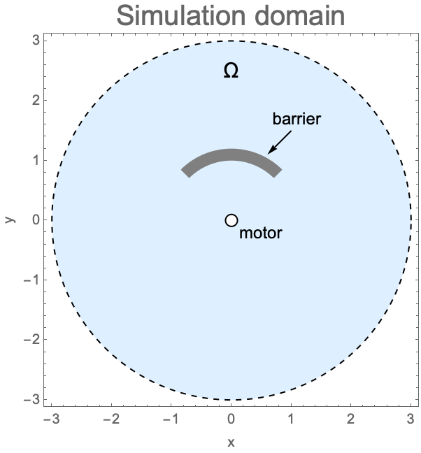
In this model the sound barrier is assumed to be made of a sound hard material, which allows it to reflect the incident sound waves. A sound hard boundary condition, which is an implicit default boundary condition, will be used to model the boundary of the barrier.