Heat Transfer Model Verification Tests
This notebook contains tests that verify that the heat transfer partial differential equations (PDE) model works as expected. To run all tests, SelectAll and press Shift+Enter. The results will then be in the section Test Result Inspection.
Note that these tests can also serve as a basis for developing your own heat transfer models. As such, the tests are grouped into stationary (time-independent) and transient (time-dependent) tests. In both categories, one- and two-dimensional test models can be found.
In each test case, the visualization section is there to provide post-processing results for inspection; however, it is not a necessary part of the test. In the interest of saving runtime and reducing memory consumption, the cells in the visualization section are set to not be evaluatable. To make these cells evaluatable, select the cells in question, choose Cell ▶ Cell Properties and make sure "Evaluatable" is ticked.
The heat equation is used to solve for the temperature field in a heat transfer model. Please refer to the information provided in "Heat Transfer" for more general theoretical background for heat transfer analysis.
$HistoryLength = 0;Stationary Tests
This section contains examples of stationary, which means non-time-dependent, heat transfer PDE models for the validation.
2D Single Equation
This section contains examples of a 2D stationary heat transfer PDE model with one equation.
HeatTransfer-FEM-Stationary-2D-Single-HeatTransfer-0001
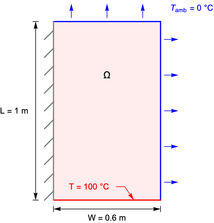
The following test case demonstrates a 2D stationary thermal analysis. The model domain ![]() is a rectangular region with a width of
is a rectangular region with a width of ![]() and a length of
and a length of ![]() . At the lower boundary, the temperature is kept at
. At the lower boundary, the temperature is kept at ![]() , and the top and right boundaries are exposed to an ambient environment with a natural convection. The remaining left boundary is thermally insulated. The ambient temperature and the heat transfer coefficient are given by
, and the top and right boundaries are exposed to an ambient environment with a natural convection. The remaining left boundary is thermally insulated. The ambient temperature and the heat transfer coefficient are given by ![]() and
and ![]() , respectively.
, respectively.
[1] A. D. Cameron, J. A. Casey and G. B. Simpson. Benchmark Tests for Thermal Analysis. NAFEMS Documentation.
For a steady-state heat transfer model without sources, the transient term ![]() and the source term
and the source term ![]() in the heat equation are set to zero. Since a solid is modeled, internal velocity
in the heat equation are set to zero. Since a solid is modeled, internal velocity ![]() also vanishes, and the heat equation simplifies to:
also vanishes, and the heat equation simplifies to:
The heat transfer coefficient and the thermal conductivity of the medium are given by ![]() and
and ![]() , respectively. The ambient temperature is held at
, respectively. The ambient temperature is held at ![]() .
.
vars = {T[x, y], {x, y}};
pars = <|"ThermalConductivity" -> 52|>;op = HeatTransferPDEComponent[vars, pars]At the point ![]() , the referenced solution [1] temperature value is given as
, the referenced solution [1] temperature value is given as ![]() .
.
ClearAll[TRef];
TRef = 18.25;The temperature at the lower boundary is fixed at ![]() .
.
Subscript[Γ, temp] = HeatTemperatureCondition[y == 0, vars, pars, <|"SurfaceTemperature" -> 100|>]The top and right boundaries are exposed to the natural convection to the ambient environment at temperature ![]() .
.
Subscript[Γ, convective] = HeatTransferValue[x == 0.6 || y == 1, vars, pars, <|"HeatTransferCoefficient" -> 750, "AmbientTemperature" -> 0|>]A default thermal insulated boundary condition is implicitly applied on the remaining left boundary.
Ω = Rectangle[{0, 0}, {0.6, 1}];pde = {op == Subscript[Γ, convective], Subscript[Γ, temp]};
measure = AbsoluteTiming[MaxMemoryUsed[Tfun = NDSolveValue[pde, T, {x, y}∈Ω]] / (1024. ^ 2)];
Print["Time -> ", measure[[1]], "
Memory -> ", measure[[2]]]VerificationTest[
RelError = (Tfun[0.6, 0.2] - TRef) / TRef;
Abs[RelError] < 10 ^ -3,
True,
TestID -> "FEM-Stationary-2D-Single-HeatTransfer-0001-A"]The following cells are marked as not evaluatable to save the runtime and memory consumed. To make these cells evaluatable, select the cells in question, choose Cell ▶ Cell Properties and make sure "Evaluatable" is ticked.
TRange = MinMax[Tfun["ValuesOnGrid"]];
legendBar = BarLegend[{"TemperatureMap", TRange}, ...];


options = {PlotRange -> TRange, ...};Legended[ContourPlot[Tfun[x, y], {x, y}∈Ω, Evaluate[options]], legendBar]HeatTransfer-FEM-Stationary-2D-Single-HeatTransfer-0002
The following test case demonstrates a 2D stationary thermal analysis. The model domain ![]() is a ceramic strip that is embedded in a high-thermal-conductivity material.
is a ceramic strip that is embedded in a high-thermal-conductivity material.
The side boundaries of the strip are maintained at a constant temperature ![]() . The top surface of the strip is losing heat via both convection and radiation to the ambient environment at
. The top surface of the strip is losing heat via both convection and radiation to the ambient environment at ![]() . The bottom boundary, however, is assumed to be thermally insulated.
. The bottom boundary, however, is assumed to be thermally insulated.

[2] J. P. Holman, Heat Transfer Tenth Edition. McGraw-Hill, pp. 111, Example 3-10 (2008).
For a steady-state heat transfer model without sources, the transient term ![]() and the source term
and the source term ![]() in the heat equation are set to zero. Since a solid is modeled, internal velocity
in the heat equation are set to zero. Since a solid is modeled, internal velocity ![]() also vanishes, and the heat equation simplifies to:
also vanishes, and the heat equation simplifies to:
The thermal conductivity ![]() , heat transfer coefficient
, heat transfer coefficient ![]() and emissivity
and emissivity ![]() of the ceramic strip are given by:
of the ceramic strip are given by:
The temperature of the left and right boundaries is held at ![]() , and the ambient temperature remains at
, and the ambient temperature remains at ![]() .
.
vars = {T[x, y], {x, y}};
pars = <|"ThermalConductivity" -> 3|>;op = HeatTransferPDEComponent[vars, pars]At points ![]() ,
, ![]() and
and ![]() , the referenced solution temperature values [3] are given by:
, the referenced solution temperature values [3] are given by:
ClearAll[TRef];
TRef = {1111.38, 1092.37, 1064.21};On the left and right boundaries, the temperature is held at ![]() .
.
Subscript[Γ, temp] = HeatTemperatureCondition[x == 0 || x == 0.02, vars, pars, <|"SurfaceTemperature" -> 1173|>]The top boundary is exposed to the environment ambient temperature ![]() , and loses heat by both thermal convection and radiation.
, and loses heat by both thermal convection and radiation.
Subscript[Γ, convective] = HeatTransferValue[y == 0.01, vars, pars, <|"HeatTransferCoefficient" -> 50, "AmbientTemperature" -> 323|>]Subscript[Γ, radiation] = HeatRadiationValue[y == 0.01, vars, pars, <|"Emissivity" -> 0.7, "AmbientTemperature" -> 323|>]A default thermal insulated boundary condition is implicitly applied on the remaining bottom boundary.
The ceramic strip has a width of ![]() and a height of
and a height of ![]() .
.
Ω = Rectangle[{0, 0}, {0.02, 0.01}];pde = {op == Subscript[Γ, convective] + Subscript[Γ, radiation], Subscript[Γ, temp]};
measure = AbsoluteTiming[MaxMemoryUsed[Tfun = NDSolveValue[pde, T, {x, y}∈Ω]] / (1024. ^ 2)];
Print["Time -> ", measure[[1]], "
Memory -> ", measure[[2]]]Tvalues = {Tfun[0.005, 0], Tfun[0.005, 0.005], Tfun[0.01, 0.005]};
VerificationTest[
Norm[(Tvalues - TRef) / TRef] < 10 ^ -2,
True,
TestID -> "FEM-Stationary-2D-Single-HeatTransfer-0002-A"]The following cells are marked as not evaluatable to save runtime and memory consumed. To make these cells evaluatable, select the cells in question, choose Cell ▶ Cell Properties and make sure "Evaluatable" is ticked.
TRange = MinMax[Tfun["ValuesOnGrid"]];
legendBar = BarLegend[{"TemperatureMap", TRange}, ...];
options = {PlotRange -> TRange, ...};Legended[ContourPlot[Tfun[x, y], {x, y}∈Ω, Evaluate[options]], legendBar]Next, calculate the rate of heat loss ![]() at the top surface of the strip. The convection and radiation heat flux
at the top surface of the strip. The convection and radiation heat flux ![]() ,
, ![]() are given by:
are given by:
bm = NDSolve`FEM`ToBoundaryMesh[Ω];
Subscript[q, conv] = NIntegrate[-Subscript[Γ, convective] /. T -> Tfun, {x, y}∈bm];


Subscript[q, rad] = NIntegrate[-Subscript[Γ, radiation] /. T -> Tfun, {x, y}∈bm];


Subscript[q, loss] = Subscript[q, conv] + Subscript[q, rad]
The heat loss rate of the ceramic strip is found as ![]() . This value can be checked by utilizing the law of energy conservation. That is, the total heat loss from the top surface must equal the conductive heat gain from the left and right boundaries:
. This value can be checked by utilizing the law of energy conservation. That is, the total heat loss from the top surface must equal the conductive heat gain from the left and right boundaries:
Subscript[q, gain] =
	Abs[NIntegrate[-k * Derivative[1, 0][Tfun][0, y] /. k -> 3, {y, 0, 0.01}]] + Abs[NIntegrate[-k * Derivative[1, 0][Tfun][0.02, y] /. k -> 3, {y, 0, 0.01}]]
Note that the heat gain value ![]() matches the rate of heat loss
matches the rate of heat loss ![]() .
.
2D Axisymmetric Single Equation
This section contains axisymmetric stationary heat transfer PDE model in cylindrical coordinates with one equation.
HeatTransfer-FEM-Stationary-2DAxisym-Single-HeatTransfer-0001
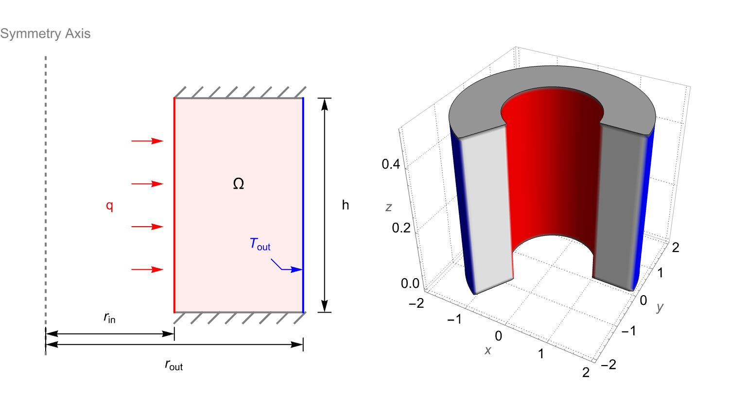
The following test case demonstrates a 2D axisymmetric steady-state thermal analysis. The model domain ![]() is a hollow cylinder with a height of
is a hollow cylinder with a height of ![]() . The inner radius and the outer radius are given by
. The inner radius and the outer radius are given by ![]() and
and ![]() , respectively. At the inner boundary, a constant heat flux
, respectively. At the inner boundary, a constant heat flux ![]() is applied to heat the domain. On the outer boundary, the temperature is held at
is applied to heat the domain. On the outer boundary, the temperature is held at ![]() . The remaining bottom and top boundaries are thermally insulated.
. The remaining bottom and top boundaries are thermally insulated.
[4] J. M. Owen and R. H. Rogers. Flow and Heat Transfer in Rotating-Disc Systems. Wiley, (1989).
For a 2D axisymmetric stationary heat transfer model without sources, the transient term ![]() and the source terms
and the source terms ![]() in the heat equation are set to zero. Since the medium is solid and the model is rotationally symmetric in the
in the heat equation are set to zero. Since the medium is solid and the model is rotationally symmetric in the ![]() direction, the terms involving the flow velocity
direction, the terms involving the flow velocity ![]() and the coordinate
and the coordinate ![]() also vanish. Then the heat equation simplifies to:
also vanish. Then the heat equation simplifies to:
vars = {T[r, z], {r, z}};
pars = <|"ThermalConductivity" -> 10, "RegionSymmetry" -> "Axisymmetric"|>;op = HeatTransferPDEComponent[vars, pars]The analytical solution of the temperature field is given by:
ClearAll[TRef];
TRef[r_, z_] := 10 * (1 - Log[r / 2])The inner boundary is subjected to a constant inward heat flux ![]() .
.
q = 100;
Subscript[Γ, flux] = NeumannValue[q, r == 1];
The temperature at the outer boundary is fixed at ![]() .
.
Subscript[Γ, temp] = DirichletCondition[T[r, z] == 10, r == 2];A default thermal insulated boundary condition is implicitly applied on the remaining bottom and top boundaries.
Ω = Rectangle[{1, 0}, {2, 1 / 2}];pde = {op == Subscript[Γ, flux], Subscript[Γ, temp]};
measure = AbsoluteTiming[MaxMemoryUsed[Tfun = NDSolveValue[pde, T, {r, z}∈Ω]] / (1024. ^ 2)];
Print["Time -> ", measure[[1]], "
Memory -> ", measure[[2]]]VerificationTest[
Norm[Table[Tfun[r, 0] - TRef[r, 0], {r, 1, 2}]] < 10 ^ -3,
True,
TestID -> "HeatTransfer-FEM-Stationary-2DAxisym-Single-HeatTransfer-0001-A"]The following cells are marked as not evaluatable to save runtime and memory consumed. To make these cells evaluatable, select the cells in question, choose Cell ▶ Cell Properties and make sure "Evaluatable" is ticked.
TRange = MinMax[Tfun["ValuesOnGrid"]];
legendBar = BarLegend[{"TemperatureMap", TRange}, ...];


options = {...};Legended[ContourPlot[Tfun[r, z], {r, z}∈Ω, Evaluate[options]], legendBar]Legended[RegionPlot3D[...], legendBar]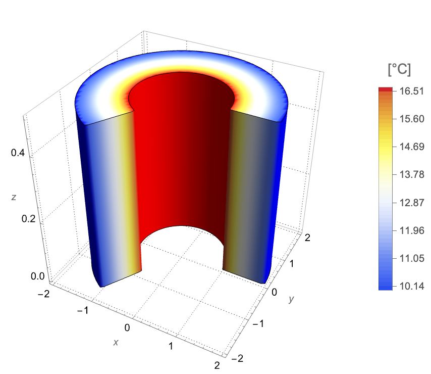
Plot[TRef[r, 0] - Tfun[r, 0], {r, 1, 2}, ...]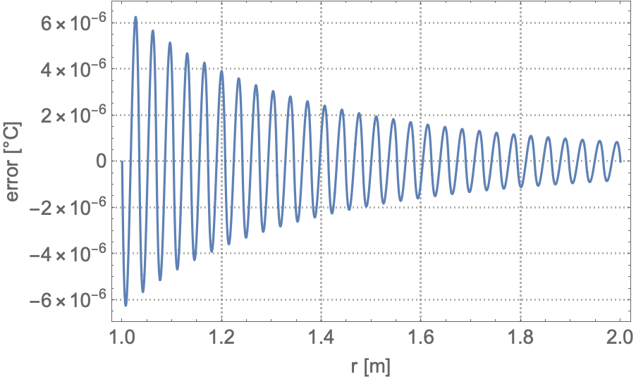
Strictly speaking, this model could be simplified further, as there is no ![]() dependency of the solution, but the original benchmark formulation is used.
dependency of the solution, but the original benchmark formulation is used.
HeatTransfer-FEM-Stationary-2DAxisym-Single-HeatTransfer-0002
This section contains a model taken from a NAFEMS benchmark collection, which shows an axisymmetric steady-state thermal analysis. The model domain ![]() is a cross section of a 3D solid hollow cylinder with a height of
is a cross section of a 3D solid hollow cylinder with a height of ![]() . The inner radius and the outer radius are given by
. The inner radius and the outer radius are given by ![]() and
and ![]() , respectively. The model is set up with three different boundary conditions: a fixed temperature condition
, respectively. The model is set up with three different boundary conditions: a fixed temperature condition ![]() at the boundaries marked with (1), a prescribed heat flux
at the boundaries marked with (1), a prescribed heat flux ![]() at (2) and an insulation/symmetry at the remaining boundaries (3).
at (2) and an insulation/symmetry at the remaining boundaries (3).

[5] A. D. Cameron, J. A. Casey and G. B. Simpson. Benchmark Tests for Thermal Analysis. NAFEMS Documentation.
For a 2D axisymmetric stationary heat transfer model without sources, the time derivative term and the source term ![]() in the heat equation are set to zero. Since the medium is solid and the model is rotationally symmetric in the
in the heat equation are set to zero. Since the medium is solid and the model is rotationally symmetric in the ![]() direction, the terms involving the flow velocity
direction, the terms involving the flow velocity ![]() and the axis
and the axis ![]() also vanish. Then the heat equation simplifies to:
also vanish. Then the heat equation simplifies to:
vars = {T[r, z], {r, z}};The material has a thermal conductivity ![]() .
.
pars = <|"ThermalConductivity" -> 52, "RegionSymmetry" -> "Axisymmetric"|>;op2D = HeatTransferPDEComponent[vars, pars]h = 0.14;
Subscript[h, 1] = 0.1;
Subscript[h, 2] = 0.04;
Subscript[r, in] = 0.02;
Subscript[r, out] = 0.1;Here ![]() and
and ![]() are the heights of the points
are the heights of the points ![]() and
and ![]() , respectively.
, respectively.
The benchmark result for the target location ![]() is a temperature of
is a temperature of ![]()
![]() .
.
ClearAll[TRef];
TRef = 332.97;The boundary ![]() is subjected to a constant inward heat flux
is subjected to a constant inward heat flux ![]() .
.
Subscript[Γ, flux] = HeatFluxValue[r == Subscript[r, in] && (Subscript[h, 2] <= z <= Subscript[h, 1]), vars, pars, <|"HeatFlux" -> 5 * 10 ^ 5|>]The temperature at the boundaries ![]() is fixed at
is fixed at ![]() .
.
Subscript[Γ, temp] = HeatTemperatureCondition[z == 0 || r == Subscript[r, out] || z == h, vars, pars, <|"SurfaceTemperature" -> 273.15|>]A default thermal insulated boundary condition is implicitly applied on the remaining boundaries ![]() .
.
Ω2D = Polygon[{{Subscript[r, in], 0.}, {Subscript[r, out], 0}, {Subscript[r, out], h}, {Subscript[r, in], h}, {Subscript[r, in], Subscript[h, 1]}, {Subscript[r, in], Subscript[h, 2]}}];measure2D = AbsoluteTiming[MaxMemoryUsed[Tfun2D = NDSolveValue[{op2D == Subscript[Γ, flux], Subscript[Γ, temp]}, T, {r, z}∈ Ω2D]] / (1024. ^ 2)];
Print["Time -> ", measure2D[[1]], "
Memory -> ", measure2D[[2]]]VerificationTest[
RelError = (Tfun2D[0.04, 0.04] - TRef) / TRef;
Abs[RelError] < 10 ^ -5,
True,
TestID -> "HeatTransfer-FEM-Stationary-2DAxisym-Single-HeatTransfer-0002-A"]Print["Error: ", 100 * (Abs[Tfun2D[0.04, 0.04] - TRef]/TRef), "%"]The solution obtained by the 2D axisymmetric approximation can be crosschecked with the solution from a 3D model.
help[{hs_, he_}] := RegionDifference@@(Cylinder[{{0, 0, hs}, {0, 0, he}}, #]& /@ {Subscript[r, out], Subscript[r, in]})
Ω3D = RegionUnion[help /@ Partition[{0, Subscript[h, 2], Subscript[h, 1], h}, 2, 1]];vars = {T[x, y, z], {x, y, z}};
pars["RegionSymmetry"] = None;measure3D = AbsoluteTiming[MaxMemoryUsed[Tfun3D = NDSolveValue[{HeatTransferPDEComponent[vars, pars] == HeatFluxValue[Sqrt[x ^ 2 + y ^ 2] == Subscript[r, in] && (Subscript[h, 2] <= z <= Subscript[h, 1]), vars, pars, <|"HeatFlux" -> 5 * 10 ^ 5|>], HeatTemperatureCondition[z == 0 || Sqrt[x ^ 2 + y ^ 2] == Subscript[r, out] || z == h, vars, pars, <|"SurfaceTemperature" -> 273.15|>]}, T, {x, y, z}∈Ω3D, Method -> {"FiniteElement", "MeshOptions" -> {"ImproveBoundaryPosition" -> True}}]] / (1024. ^ 2)];
Print["Time -> ", measure3D[[1]], "
Memory -> ", measure3D[[2]]]Since there is a symbolic description of the region, the option "ImproveBoundaryPosition" can be used for 3D geometries to further improve the boundary shape of the mesh.
VerificationTest[
	RelError = (Tfun3D[0.04, 0, 0.04] - TRef) / TRef;
	Abs[RelError] < 10 ^ -3,
	True,
TestID -> "HeatTransfer-FEM-Stationary-2DAxisym-Single-HeatTransfer-0002-B"]Print["Error: ", 100 * (Abs[Tfun3D[0.04, 0, 0.04] - TRef]/TRef), "%"]The following cells are marked as not evaluatable to save runtime and memory consumed. To make these cells evaluatable, select the cells in question, choose Cell ▶ Cell Properties and make sure "Evaluatable" is ticked.
ContourPlot[Tfun2D[r, z], {r, z}∈Ω2D, ...]Legended[RegionPlot3D[Subsuperscript[r, in, 2] ≤ x^2 + y^2 ≤ Subsuperscript[r, out, 2] && 0 ≤ PlanarAngle[{0, 0} -> {{Subscript[r, in], 0}, {x, y}}] ≤ (4 π/3), {x, -Subscript[r, out], Subscript[r, out]}, {y, -Subscript[r, out], Subscript[r, out]}, {z, 0, h}, ...], BarLegend[...]]Transient Tests
This section contains examples of transient (time-dependent) heat transfer PDE models for validation.
1D Single Equation
This section contains examples of transient heat transfer ordinary differential equations (ODE) models with one equation. Ordinary differential equations with one independent variable are a special case of partial differential equations that usually deal with more than one independent variable.
HeatTransfer-FEM-Transient-1D-Single-HeatTransfer-0001
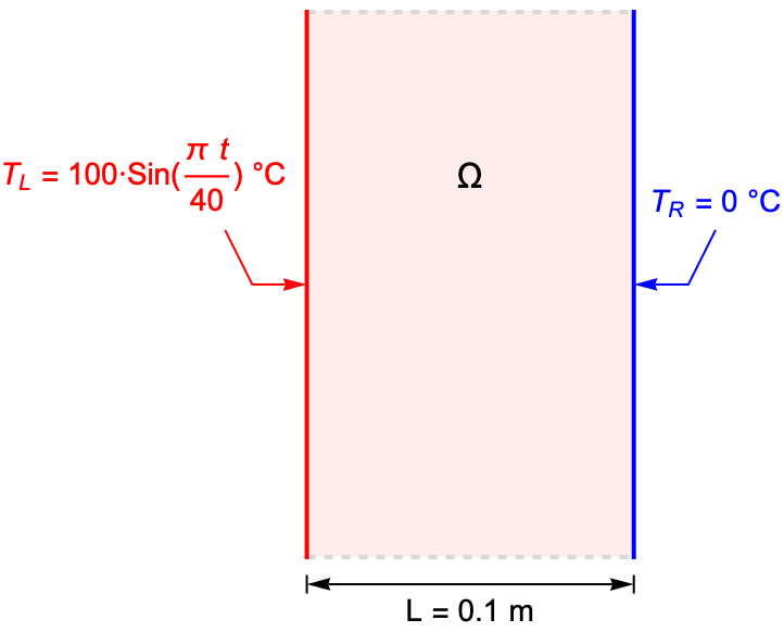
The following test case shows a transient heat diffusion process within a plate. The temperature ![]() on the left surface varies sinusoidally in time; on the other surface, the temperature is fixed at
on the left surface varies sinusoidally in time; on the other surface, the temperature is fixed at ![]() . It is assumed that the plate is very large compared to its thickness, so the analysis reduces to a 1D heat transfer model along the thickness.
. It is assumed that the plate is very large compared to its thickness, so the analysis reduces to a 1D heat transfer model along the thickness.
[6] A. D. Cameron, J. A. Casey and G. B. Simpson. Benchmark Tests for Thermal Analysis. NAFEMS Documentation.
For a transient heat transfer model in a solid without sources, the source term ![]() and the internal velocity
and the internal velocity ![]() in the heat equation are set to zero. The heat equation then simplifies to:
in the heat equation are set to zero. The heat equation then simplifies to:
The density, heat capacity and thermal conductivity of the medium are given by ![]() ,
, ![]() and
and ![]() , respectively.
, respectively.
vars = {T[t, x], t, {x}};
pars = <|"ThermalConductivity" -> 35, "MassDensity" -> 7200, "SpecificHeatCapacity" -> 440.5|>;op = HeatTransferPDEComponent[vars, pars]At time ![]() , the referenced solution [1] of the temperature at point
, the referenced solution [1] of the temperature at point ![]() is given as
is given as ![]() .
.
ClearAll[TRef];
TRef = 36.6;On the left surface, the plate experiences a transient heating, where the temperature varies sinusoidally in time by ![]()
![]() . On the right surface, the temperature is held at
. On the right surface, the temperature is held at ![]() .
.
Subscript[Γ, tempL] = HeatTemperatureCondition[x == 0, vars, pars, <|"SurfaceTemperature" -> 100Sin[π t / 40]|>]
Subscript[Γ, tempR] = HeatTemperatureCondition[x == 0.1, vars, pars]At time ![]() , the temperature of the plate is
, the temperature of the plate is ![]() .
.
ic = {T[0, x] == 0};The thickness of the plate is given by ![]() .
.
Ω = Line[{{0}, {0.1}}];tend = 32;pde = {op == 0, Subscript[Γ, tempL], Subscript[Γ, tempR], ic};
measure = AbsoluteTiming[MaxMemoryUsed[Tfun = NDSolveValue[pde, T, {t, 0, tend}, {x}∈Ω]] / (1024. ^ 2)];
Print["Time -> ", measure[[1]], "
Memory -> ", measure[[2]]]VerificationTest[
RelError = (Tfun[tend, 0.02] - TRef) / TRef;
RelError < 10 ^ -3,
True,
TestID -> "HeatTransfer-FEM-Transient-1D-Single-HeatTransfer-0001-A"]The following cells are marked as not evaluatable to save runtime and memory consumed. To make these cells evaluatable, select the cells in question, choose Cell ▶ Cell Properties and make sure "Evaluatable" is ticked.
nframes = 30;
frames = Table[Plot[Tfun[t, x], x∈Ω, ...], {t, 0, tend, tend / nframes}];
ListAnimate[...]
HeatTransfer-FEM-Transient-1D-Single-HeatTransfer-0002
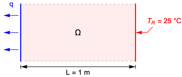
The following test case demonstrates a transient heat diffusion within a rod. On the left end, a constant outward heat flux ![]() is set to simulate the cooling process. On the right end, the temperature is fixed at
is set to simulate the cooling process. On the right end, the temperature is fixed at ![]() .
.
[7] H. S. Carslaw and J. C. Jaeger. Conduction of Heat in Solids. Oxford at the Clarendon Press, 2nd ed. (1959).
For a transient heat transfer model in a solid without sources, the source term ![]() and the internal velocity
and the internal velocity ![]() in the heat equation are set to zero. The heat equation then simplifies to:
in the heat equation are set to zero. The heat equation then simplifies to:
The density, heat capacity and thermal conductivity of the medium are given by ![]() ,
, ![]() and
and ![]() , respectively.
, respectively.
vars = {T[t, x], t, {x}};
pars = <|"ThermalConductivity" -> 1, "MassDensity" -> 1, "SpecificHeatCapacity" -> 1|>;op = HeatTransferPDEComponent[vars, pars]The analytical solution of the temperature field is given by:
ClearAll[TRef];
TRef[t_, x_] := (24 + x) + 8 / π^2 * Cos[π / 2 * x] * Exp[-π^2 / 4 * t] + 8 / 9 / π^2 * Cos[3π / 2 * x] * Exp[-(9 / 4 * π^2) * t]The left end is losing heat at a constant outward heat flux ![]() .
.
Subscript[Γ, flux] = HeatFluxValue[x == 0, vars, pars, <|"HeatFlux" -> -1|>]The temperature at the right end is fixed at ![]() .
.
Subscript[Γ, temp] = HeatTemperatureCondition[x == 1, vars, pars, <|"SurfaceTemperature" -> 25|>]At time ![]() , the temperature of the plate is
, the temperature of the plate is ![]() .
.
ic = {T[0, x] == 25};The model domain ![]() is a rod with a length of
is a rod with a length of ![]() .
.
Ω = Line[{{0}, {1}}];tend = 0.2;pde = {op == Subscript[Γ, flux], Subscript[Γ, temp], ic};
measure = AbsoluteTiming[MaxMemoryUsed[Tfun = NDSolveValue[pde, T, {t, 0, tend}, {x}∈Ω]] / (1024. ^ 2)];
Print["Time -> ", measure[[1]], "
Memory -> ", measure[[2]]]VerificationTest[
Norm[Table[Tfun[tend, x] - TRef[tend, x], {x, 0, 1}]] < 10 ^ -3,
True,
TestID -> "HeatTransfer-FEM-Transient-1D-Single-HeatTransfer-0002-A"]The following cells are marked as not evaluatable to save runtime and memory consumed. To make these cells evaluatable, select the cells in question, choose Cell ▶ Cell Properties and make sure "Evaluatable" is ticked.
nframes = 30;
frames = Table[Plot[Tfun[t, x], x∈Ω, ...], {t, 0, tend, tend / nframes}];
ListAnimate[...]Plot[TRef[tend, x] - Tfun[tend, x], x∈Ω, ...]2D Axisymmetric Single Equation
This section contains an axisymmetric transient heat transfer PDE model in cylindrical coordinates with one equation.
HeatTransfer-FEM-Transient-2DAxisym-Single-HeatTransfer-0001
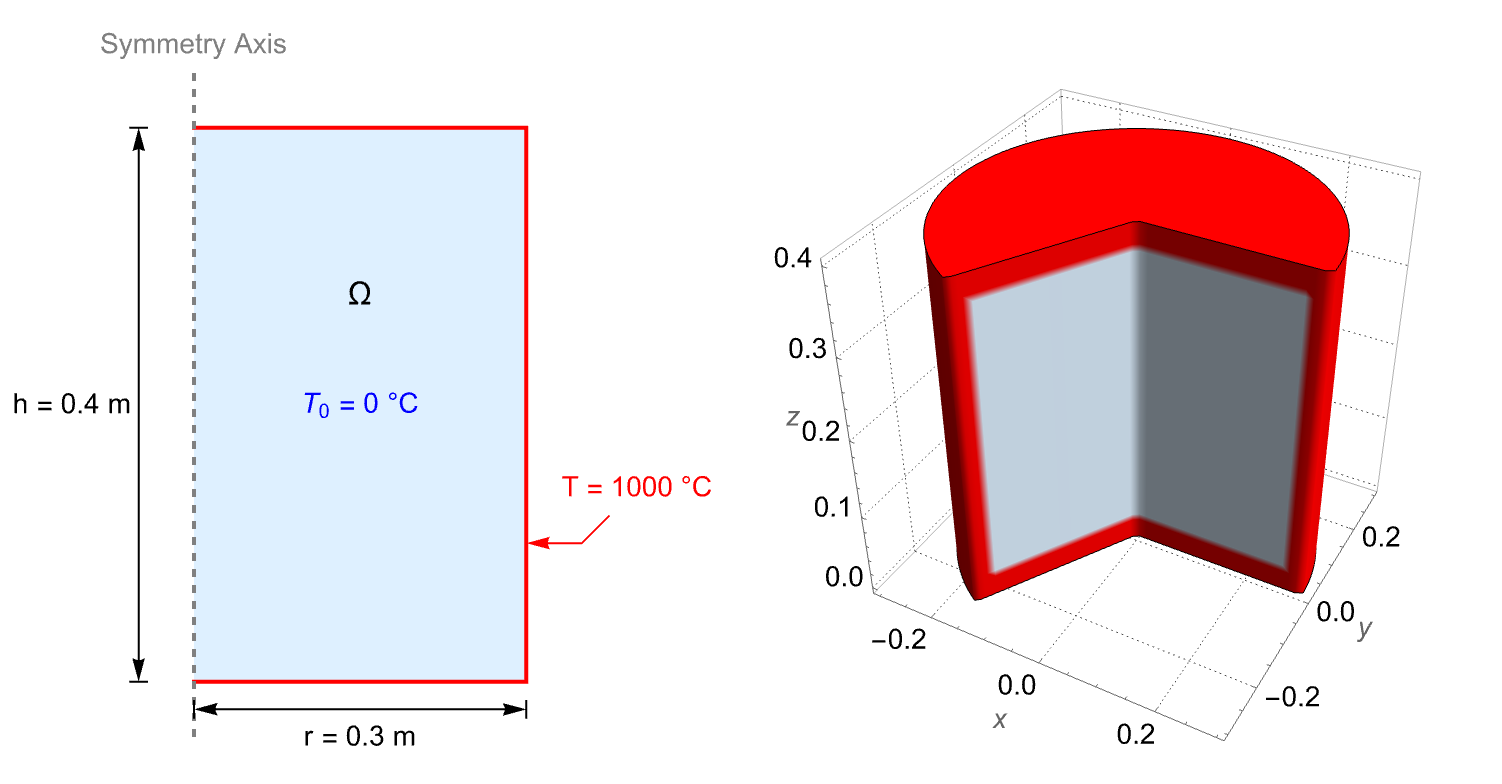
The following test case demonstrates a 2D axisymmetric transient thermal analysis. The model domain ![]() is a cylinder with a radius of
is a cylinder with a radius of ![]() and a height of
and a height of ![]() . The temperature of the entire domain begins at
. The temperature of the entire domain begins at ![]() . At the outer boundaries, the temperature experiences a step jump to and stays at
. At the outer boundaries, the temperature experiences a step jump to and stays at ![]() for
for ![]() .
.
[8] A. D. Cameron, J. A. Casey and G. B. Simpson. Benchmark Tests for Thermal Analysis. NAFEMS Documentation.
When modeling the heat transfer in a solid medium without sources, the internal velocity ![]() and the source
and the source ![]() in the heat equation are set to zero. Since the model is rotationally symmetric in the
in the heat equation are set to zero. Since the model is rotationally symmetric in the ![]() direction, the terms involving the coordinate
direction, the terms involving the coordinate ![]() also vanish. Then the heat equation simplifies to:
also vanish. Then the heat equation simplifies to:
vars = {T[t, r, z], t, {r, z}};The density, heat capacity and thermal conductivity of the medium are given by ![]() ,
, ![]() and
and ![]() , respectively.
, respectively.
pars = <|"ThermalConductivity" -> 52, "MassDensity" -> 7850, "SpecificHeatCapacity" -> 460, "RegionSymmetry" -> "Axisymmetric"|>;op = HeatTransferPDEComponent[vars, pars]At ![]() , the referenced solution [1] temperature value at the point
, the referenced solution [1] temperature value at the point ![]() is given as
is given as ![]() .
.
ClearAll[TRef];
TRef = 186.5;The temperature at the outer boundary is fixed at ![]() .
.
Subscript[Γ, temp] = DirichletCondition[T[t, r, z] == 1000, r == 0.3 || z == 0 || z == 0.4];At time ![]() , the temperature of the domain is
, the temperature of the domain is ![]() .
.
ic = {T[0, r, z] == 0};Ω = Rectangle[{0, 0}, {0.3, 0.4}];tend = 190;pde = {op == 0, Subscript[Γ, temp], ic};
measure = AbsoluteTiming[MaxMemoryUsed[Tfun = NDSolveValue[pde, T, {t, 0, tend}, {r, z}∈Ω]] / (1024. ^ 2)];
Print["Time -> ", measure[[1]], "
Memory -> ", measure[[2]]]VerificationTest[
RelError = (Tfun[190, 0.1, 0.3] - TRef) / TRef;
Abs[RelError] < 10 ^ -2,
True,
TestID -> "HeatTransfer-FEM-Transient-2DAxisym-Single-HeatTransfer-0001-A"]The following cells are marked as not evaluatable to save runtime and memory consumed. To make these cells evaluatable, select the cells in question, choose Cell ▶ Cell Properties and make sure "Evaluatable" is ticked.
TRange = MinMax[Tfun["ValuesOnGrid"]];
legendBar = BarLegend[{"TemperatureMap", TRange}, ...];


options = {PlotRange -> TRange, ...};nframes = 30;
frames = Table[Legended[ContourPlot[Tfun[t, r, z], {r, z}∈Ω, Evaluate[options]], legendBar], {t, 0, tend, tend / nframes}];
frames = Map[...];
ListAnimate[...]See this note about improving the visual quality of the animation.
Legended[RegionPlot3D[...], legendBar]Test Result Inspection
This section contains the evaluation of the test runs. It works by collecting all instances of TestResultObject and generating a TestReport.
nb = EvaluationNotebook[];
cso = Cells[nb, CellStyle -> {"Output"}];
tros = Cases[ToExpression[First[NotebookRead[#]]]& /@ cso, _TestResultObject];
report = TestReport[tros]Column /@ (Normal /@ report["TestsFailed"])//TabViewIf the preceding table is empty, all tests succeeded.
References
1. A. D. Cameron, J. A. Casey and G. B. Simpson. Benchmark Tests for Thermal Analysis. NAFEMS Documentation.
2. J. M. Owen and R. H. Rogers. Flow and Heat Transfer in Rotating-Disc Systems. Wiley, (1989).
3. H. S. Carslaw and J. C. Jaeger. Conduction of Heat in Solids. Oxford at the Clarendon Press, 2nd ed. (1959).
4. J. P. Holman, Heat Transfer Tenth Edition. McGraw-Hill, pp. 111, Example 3-10 (2008).