Inductive Heating
Inductive heating is a process in which a material is heated up due to currents that flow in the material. This process is similar to the Joule heating effect, but the currents that heat the material are induced by means of an electromagnetic induction. The main characteristic of this heating process is that is a contactless process.
The basic components of an inductive heating system are a coil and a workpiece that is placed inside the coil, without touching it. An alternating current is applied to the coil and a time-varying magnetic field is generated. Then, the alternating electromagnetic field induces eddy currents in the workpiece, resulting in resistive losses, which leads to a rise of temperature.
Most commonly, these types of models are simulated using a one-way approach. This type of approach is also called a segregated simulation. In this approach, a magnetic quasistatic frequency study is performed first and then followed by a transient heat transfer study. This is based on the assumption that changes in the magnetic field—the magnetic cycle time—occur much more rapidly than changes in temperature, known as the thermal time scale. This allows the problem to be treated as adiabatic, meaning heat is generated internally without significant loss to the surroundings during the magnetic cycle time. A fully coupled model should be made use of if the electrical conductivity of the material is considered to be temperature dependent, which is not done here.
The magnetic quasistatic frequency study is based on the following equation:
where ![]() is the vacuum permeability in units of [
is the vacuum permeability in units of [![]() ],
], ![]() is the unitless relative permeability, and
is the unitless relative permeability, and ![]() is the electrical conductivity in units of [
is the electrical conductivity in units of [![]() ].
]. ![]() is the magnetic vector potential in units of [
is the magnetic vector potential in units of [![]() ], and
], and ![]() is the external electric current density vector in units of [
is the external electric current density vector in units of [![]() ]. This equation can be generated by MagneticPDEComponent and by specifying an angular frequency variable
]. This equation can be generated by MagneticPDEComponent and by specifying an angular frequency variable ![]() [
[![]() ].
].
A heat source ![]() [
[![]() ] can be computed from the magnetic vector potential
] can be computed from the magnetic vector potential ![]() , and that heat source will then be used in a heat transfer model. The heat source, in fact, depends on the secondary
, and that heat source will then be used in a heat transfer model. The heat source, in fact, depends on the secondary ![]() ,
, ![]() and
and ![]() fields derived from the magnetic vector potential
fields derived from the magnetic vector potential ![]() , which is the solution from the quasistatic magnetic model. The heat source represents the time average of the inductive heating over one period and is given by:
, which is the solution from the quasistatic magnetic model. The heat source represents the time average of the inductive heating over one period and is given by:
where ![]() [
[![]() ] are the resistive losses and
] are the resistive losses and ![]() [
[![]() ] are the magnetic losses. The fields are complex valued, where
] are the magnetic losses. The fields are complex valued, where ![]() is the complex conjugate of
is the complex conjugate of ![]() and
and ![]() is the complex conjugate of
is the complex conjugate of ![]() .
. ![]() is the imaginary unit and
is the imaginary unit and ![]() is the angular frequency [
is the angular frequency [![]() ].
].
After the magnetic quasistatic frequency study is performed and the heat source computed, then one can move forward to perform a transient heat transfer study.
The heat source ![]() previously defined enters the transient heat equation by:
previously defined enters the transient heat equation by:
The dependent variable in the heat equation is the temperature ![]() , which varies with time
, which varies with time ![]() and position
and position ![]() . The partial differential equation (PDE) model describes how thermal energy is transported over time in a medium with density
. The partial differential equation (PDE) model describes how thermal energy is transported over time in a medium with density ![]() and specific heat capacity
and specific heat capacity ![]() . The specific heat capacity is a material property that specifies the amount of heat energy that is needed to raise the temperature of a substance with unit mass by one degree Kelvin. Besides the time derivative part, the PDE is made up of several components. First and foremost, there is a diffusive term:
. The specific heat capacity is a material property that specifies the amount of heat energy that is needed to raise the temperature of a substance with unit mass by one degree Kelvin. Besides the time derivative part, the PDE is made up of several components. First and foremost, there is a diffusive term: ![]() with a thermal conductivity
with a thermal conductivity ![]() . There is no convective component in this case.
. There is no convective component in this case.
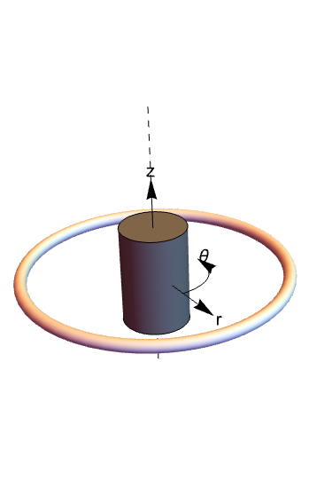
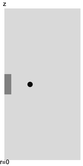
In the heat inductance model, a copper cylinder is placed inside a single copper coil, and the coil is excited at a frequency of 500 [![]() ]. The model will be approximated with a 2D axisymmetric formulation.
]. The model will be approximated with a 2D axisymmetric formulation.
On the left: a simulation domain of a 3D cylinder placed inside a 3D coil in a cylindrical coordinate system. To the right: a cross-sectional area of the coil and cylinder and its surrounding volume in the![]() -
-![]() plane.
plane.
First, a magnetic quasistatic frequency simulation will be performed, and for that, material parameters and variables need to be defined.
Copper has an electrical conductivity of ![]() and air an electrical conductivity of zero and both have a relative permeability of 1.
and air an electrical conductivity of zero and both have a relative permeability of 1.
In the next part, the heat source is defined.
Next, the heat transfer model is set up.
The heat transfer model will be performed only in the conductor region.
At the boundary, at ![]() , a heat symmetry condition will be applied, as it is the axis of symmetry. A HeatSymmetryValue produces a Neumann 0 value. As these are the natural default boundary conditions, these can be left out.
, a heat symmetry condition will be applied, as it is the axis of symmetry. A HeatSymmetryValue produces a Neumann 0 value. As these are the natural default boundary conditions, these can be left out.
The model is simulated from time 0 to 10 hours.
The plot on the left shows how the workpiece starts to heat, and the plot on the right shows the temperature distribution after 36,000 seconds. In addition, the maximum and minimum values of both plots are very close, so it can be concluded that the temperature is almost constant over the whole workpiece in each time step.

