Solid Mechanics Model Verification Tests

Stationary Tests	Test Result Inspection
Eigenmode Analysis Tests

The solid mechanics PDE components are in experimental stage.

This notebook contains tests that verify that the solid mechanics partial differential equations (PDE) model works as expected. To run all tests, SelectAll and press Shift+Enter. The results will then be in the section Test Result Inspection.

Note that these tests can also serve as a basis for developing your own solid mechanics models. As such, the tests are grouped into stationary (time-independent) and transient (time-dependent) tests. In both categories, two- and three-dimensional tests can be found.

In each test case the visualization section is there to provide post-processing results for inspection, however, it is not a necessary part of the test. In the interest of saving runtime and reducing memory consumption the cells in the visualization section are set to not be evaluatable. To make these cells evaluatable, select the cells in question and choose Cell ▶ Cell Properties and make sure "Evaluatable" is ticked.

The solid mechanics equations are used to solve for the displacement of a constrained object under load. Please refer to the information provided in "Solid Mechanics" for a more general theoretical background for solid mechanics analysis.

Load the finite element package:

To avoid keeping memory intensive previous results set the history length to 0:

A helper function to visualize deformation of structures under load:

Stationary Tests

This section contains examples of stationary (non-time-dependent) solid mechanics PDE models for the validation.

2D Equations

This section contains examples of 2D stationary solid mechanics PDE models.

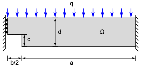
SolidMechanics-FEM-Stationary-2D-PlaneStress-0001

The following test cases verify various aspects of 2D plane stress analysis. The model domain is a notched beam with a total width of , a height of and thickness . At the left boundary a roller constraint is present and the structure is fixed at the right hand side. A pressure of is acting in a downward direction on the top. The remaining boundaries are free to move. Young's modulus is given as and Poisson's ratio is .

Test Reference:

M. Asghar Bhatti. Fundamental Finite Element Analysis and Applications. Wiley., Page 510, Example 7.7, Notched Beam

M. Asghar Bhatti. Fundamental Finite Element Analysis and Applications. Wiley. Supplementary examples from Book web page, Page 34, Chapter 7, Notched Beam

Equation:

The standard plane stress model is used.

Define the model variables and parameters:

Set up a 2D steady-state solid mechanics model:

Set up a second 2D steady-state solid mechanics model that uses stress and strain functions:

Solution:

The nodal displacements are given.

Specify the reference nodal displacements:

Boundary Conditions:

The structure is held fixed at the right hand side.

Fix the structure at the right hand side:

The structure is attached to a roller in the y-direction on the left.

A roller on the left in the y-direction

On the top a pressure of 50 units is applied in the downward direction.

Set up a boundary load acting on the top:

The remaining sides are free to move.

Region:

Set up the model region:

Test 1:

Solve the PDE model and monitor time/memory usage:

Test the inactive PDE:

Test 2:

Solve the PDE model and monitor time/memory usage:

Test the inactive PDE:

Test 3:

Verify the material model:

Test 4:

Compute the reaction force:

Verify the reaction force:

Visualization:

The following cells are marked as not evaluatable to save the runtime and consume memory. To make these cells evaluatable, select the cells in question and choose Cell ▶ Cell Properties and make sure "Evaluatable" is ticked.

Visualize the deformed structure:

Comment:

Bhatti's example goes further and computes various stresses. Bhatti's example exclusively is based on linear elements. In the Wolfram language, however, a special techniques is used to have a higher order interpolation also in the linear element case and special algorithms to recover derivatives. Thus the stress values computed with the Wolfram language and the simplistic (yet instructive) example of Bhatti's do not match and are not shown here.

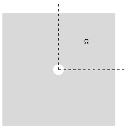
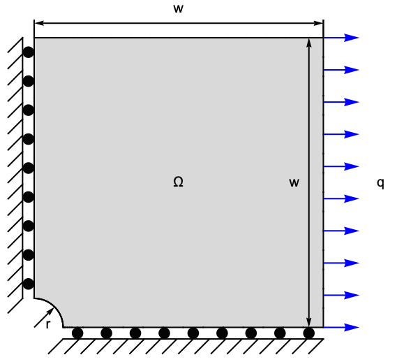
SolidMechanics-FEM-Stationary-2D-PlaneStress-0002

The following test case verifies 2D plane stress analysis and computes stresses to be compared with an analytical solution. The original model is for an infinite plate with a hole inside. To simulate this model the domain is made finite and is a quarter symmetry of the rectangular plate with a quarter hole at the lower left corner.

The modeled plate has a width of , a height of also and thickness . The radius of the hole is . At the left boundary a roller constraint is used such that the structure can move up or down but not to the right. At the bottom there is a second roller constraint such that the structure can move left to right but not up and down. A pressure of is acting in the x-direction on the right hand side. The remaining boundaries are free to move. Young's modulus is not needed and assumed as and Poisson's ratio is .

Test Reference:

D. Roylance, Mechanics of Materials, Wiley., Page 184

Equation:

The standard plane stress model is used.

Define the model variables and parameters:

Set up a 2D steady-state solid mechanics model:

Set up a second 2D steady-state solid mechanics model that uses stress and strain functions:

Solution:

An expression for the stress in x-direction is given

Specify the referenced stress function with values:

Boundary Conditions:

The structure is held fixed at the right hand side.

A roller constraint at the bottom in the y-direction

The structure is attached to a roller in the y-direction on the left.

A roller constraint at the left in the x-direction

On right a pressure of 1000 [Pa] is applied in the downward positive x-direction.

Set up a boundary load acting on the right in the x-direction:

The remaining sides are free to move.

Region:

Set up the model region:

Test 1:

Solve the PDE model and compute the stress:

Test the stress PDE:

Test 2:

Solve the PDE model and compute the stress on a refined mesh:

Test 3:

Solve the PDE model and compute the stress:

Test the inactive PDE:

Test 4:

Solve the PDE model and compute the stress:

Test the inactive PDE:

Visualization:

Plot analytical and computed stress.

Plot the relative percent error of the computed stress.

Comment:

Aside from the expected deviation at the end, the analytical and simulated results match closely. The deviation at the end is expected because the analytical model is for an infinite plate that isn't modeled here. Enlarging the domain by setting will further improve the quality of the solution.

SolidMechanics-FEM-Stationary-2D-PlaneStress-0003

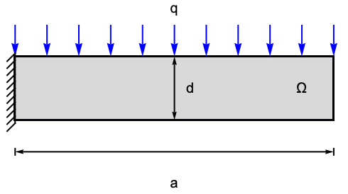
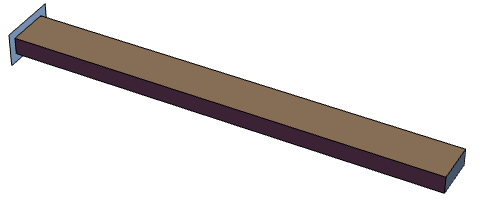
The following test case verifies a 2D plane stress analysis of a beam. The model domain is a beam with a total width of , a height of and thickness . At the left boundary the beam is fixated to a wall. A pressure of is acting in a downward direction on the top. The remaining boundaries are free to move. Young's modulus is given as and Poisson's ratio is . The mass density is given as .

Test Reference:

G. Backstrom, Simple displacement and Vibration, GB Publishing, 2006, ISBN: 9-1975553-20, Page 59

Equation:

The standard plane stress model is used.

Define the model variables and parameters:

Set up a 2D steady-state solid mechanics model:

Set up a second 2D steady-state solid mechanics model that uses stress and strain functions:

Solution:

The nodal displacements are given.

Specify the reference nodal displacements:

Boundary Conditions:

The structure is held fixed at the left hand side.

Fix the structure at the left hand side:

On the top a pressure of 10^6 units is applied in the downward direction.

Set up a boundary load acting on the top:

The remaining sides are free to move.

Region:

Set up the model region:

Test 1:

Solve the PDE model and monitor time/memory usage:

Test the inactive PDE:

Test 2:

Solve the PDE over a triangle mesh:

Test the inactive PDE:

Test 3:

Solve the PDE model and monitor time/memory usage:

Test the inactive PDE:

Test 4:

Solve the PDE model and monitor time/memory usage:

Test the inactive PDE:

Visualization:

Visualize the deformed structure:

Plot the analytical solution of the vertical displacement versus the numerical solution

SolidMechanics-FEM-Stationary-2D-PlaneStress-0004

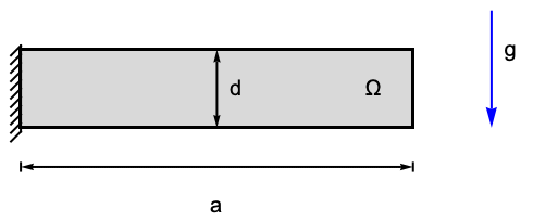
The following test case verifies a 2D plane stress analysis of a beam. The model domain is a beam with a total width of , a height of and thickness . At the left boundary the beam is fixated to a wall. The remaining boundaries are free to move. Gravity acts on the body. Young's modulus is given as and Poisson's ratio is . The mass density is given as .

Test Reference:

G. Backstrom, Simple displacement and Vibration, GB Publishing, 2006, ISBN: 9-1975553-20, Page 68

Equation:

The standard plane stress model is used.

Define the model variables and parameters:

Set up a 2D steady-state solid mechanics model:

Set up a second 2D steady-state solid mechanics model that uses stress and strain functions:

Solution:

The nodal displacements are given.

Specify the reference nodal displacements:

Boundary Conditions:

The structure is held fixed at the left hand side.

Fix the structure at the left hand side:

The remaining sides are free to move.

Region:

Set up the model region:

Test 1:

Solve the PDE model and monitor time/memory usage:

Test the inactive PDE:

Test 2:

Solve the PDE over a triangle mesh:

Test the inactive PDE:

Test 3:

Solve the PDE model and monitor time/memory usage:

Test the inactive PDE:

Test 4:

Solve the PDE model and monitor time/memory usage:

Test the inactive PDE:

Visualization:

Visualize the deformed structure:

Plot the analytical solution of the vertical displacement versus the numerical solution

SolidMechanics-FEM-Stationary-2D-PlaneStress-0005

The model domain is a beam with a total length of , a height of and thickness . At the right boundary the beam is fixated to a wall. The remaining boundaries are free to move. Young's modulus is given as and Poisson's ratio is , which makes this compatible with beam theory. The maximal bending stress at middle of the beam ( and the fixated end ( are sought.

Test Reference:

S. H. Crandall, N. C. Dahl, An Introduction to the Mechanics of Solids, McGraw-Hill Book Co., Inc., New York, NY, 1959, pg. 342, problem 7.18.

Equation:

The standard stress model with a thickness specified is used.

Define the model variables and parameters:

Set up a 2D steady-state solid mechanics model:

Solution:

The maximum bending stress at mid length and the fixated end are sought.

Specify the reference values:

Boundary Conditions:

The beam is fixed at the right hand side.

Fix the structure at the right hand side and apply a load:

Region:

Set up the model region:

Visualize the mesh:

Solve:

Solve the PDE model and monitor time/memory usage:

Test 1:

Test the first solution:

Test 2:

Test the second solution:

Test 3:

Test the third solution:

Test 4:

Test the fourth solution:

Visualization:

Visualize the deformed structure:

SolidMechanics-FEM-Stationary-2D-PlaneStress-0006

The model domain is a beam with a total length of , a height of and thickness . At the left boundary the beam is fixated to a wall. At the right there are two load test cases: Case 1 is a bending moment and case 2 is an upward force. The remaining boundaries are free to move. Young's modulus is given as and Poisson's ratio is . For each test case the deflection at the free and is sought and the bending stress at a distance from the fixation at the left.

Test Reference:

R. J. Roark, Formulas for Stress and Strain, 4th Edition, McGraw-Hill Book Co., Inc., New York, NY, 1965, pp. 104, 106.

Equation:

The standard stress model is used.

Define the model variables and parameters:

Set up a 2D steady-state solid mechanics model:

Solution:

Reference values are given:

Specify the reference values:

Boundary Conditions:

The beam is fixed at the left hand side.

Fix the structure at the left hand side:

Region:

Set up the model region:

Visualize the mesh:

Solve:

Solve the PDE model and monitor time/memory usage:

Test 1:

Test the first solution:

Test 2:

Test the second solution:

Test 3:

Test the first displacement:

Test 4:

Test the second displacement:

Test 5:

Test the first displacement:

Visualization:

Visualize the deformed structure:

SolidMechanics-FEM-Stationary-2D-PlaneStress-0007

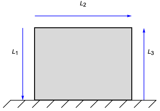
A rectangular plate is fixed at the bottom. Three boundary loads are applied on the left, top and right such that the normal strains vanish and the shear strain is constant.

Test Reference:

G. Backstrom, Simple displacement and Vibration, GB Publishing, 2006, ISBN: 9-1975553-20, Page 56

Equation:

The standard plane stress model is used.

Define the model variables and parameters:

Set up a 2D steady-state solid mechanics models:

Solution:

Reference values are given:

Specify the reference values:

Boundary Conditions:

The plate is fixed at the bottom and pressures or forces are applied at the remaining boundaries.

Fix the structure at the bottom:

Apply pressures:

Fix the structure at the bottom and apply forces:

Region:

Set up the model region:

Solve:

Solve the PDE models:

Test 1:

Test the first solution:

Test 2:

Test the second solution:

Test 3:

Test the third solution:

Test 4:

Test the fourth solution:

Visualization:

Visualize the deformed structure:

SolidMechanics-FEM-Stationary-2D-PlaneStrain-0001

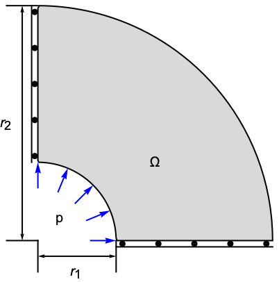
The following test cases verify various aspects of 2D plane strain analysis. The model domain is a quarter cross section through a pipe with an inner radius an outer radius and a thickness . At the left boundary a symmetry constraint is used such that the pipe can move up and down and at the right bottom a second symmetry constraint is used such that the pipe can move left and right. A pressure of is acting within the pipe. The remaining boundaries are free to move. Young's modulus is given as and Poisson's ratio is .

Test Reference:

M. Asghar Bhatti. Fundamental Finite Element Analysis and Applications. Wiley., Page 517, Example 7.9, Pressure Vessels

Equation:

The standard plane strain model is used.

Define the model variables and parameters:

Set up a 2D steady-state solid mechanics model:

Set up a second 2D steady-state solid mechanics model that uses stress and strain functions:

Solution:

The tangential and radial stresses are given.

Specify the analytical reference solution:

Boundary Conditions:

The quarter pipe structure exploits a symmetry condition y-direction on the left.

A symmetry condition on the left in the y-direction:

A symmetry condition on the bottom in the x-direction:

Inside a pressure of 20 units is applied in the outward direction.

Set up a boundary load acting inside on an outward direction:

The remaining sides are free to move.

Region:

Set up the model region:

Test 1:

Solve the PDE and compute the strain and stress:

Verify the tangential stress:

Test 2:

Verify the tangential stress:

Test 3:

Solve the PDE and compute the strain and stress:

Verify the tangential stress:

Test 4:

Verify the tangential stress:

Visualization:

Visualize the deformed structure:

3D Equations

This section contains examples of 3D stationary solid mechanics PDE models.

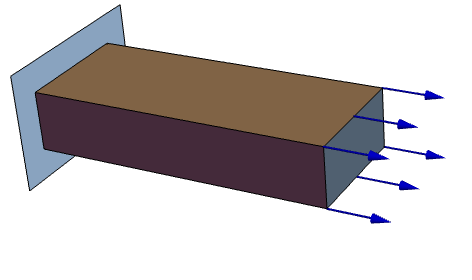
SolidMechanics-FEM-Stationary-3D-0001

The following test cases verify a 3D stress analysis. The model domain is a beam with a length of , a width of , a height of . At the left boundary the beam is fixed to a wall. At the right hand side a force of is acting in the direction. The remaining boundaries are free to move. As a material a S235 steel is used. Thus Young's modulus is given as and Poisson's ratio is .

Test Reference:

M. Brand, Grundlagen FEM mit Solidworks, Vieweg+Teuber, 2011, ISBN: 978-3-8348-1306-0, Page 7

Equation:

The standard stress model is used.

Define the model variables and parameters:

Set up a 3D steady-state solid mechanics model:

Set up a second 3D steady-state solid mechanics model that uses stress and strain functions:

Solution:

An expected elongation in the direction of is given. Inside the domain a stress of is given. The elongation can be computed with

It follows that

The stress in is computed to be

Specify the reference values:

Boundary Conditions:

The structure is held fixed at the left hand side.

Fix the structure at the left hand side:

On the right hand side a force of acts in the direction.

Set up a force acting on the right boundary in the

direction.

The remaining sides are free to move.

Region:

Set up the model region and meshes with hexahedron and tetrahedron elements.

Visualize the mesh:

Solve the PDE model and monitor time/memory usage:

Compute stress and strain.

Solve the PDE model and monitor time/memory usage:

Compute stress and strain.

Solve the PDE model and monitor time/memory usage:

Compute stress and strain.

Solve the PDE model and monitor time/memory usage:

Compute stress and strain.

Test 1:

Test the first PDE on the first mesh:

Test 2:

Test the second PDE on the first mesh:

Test 3:

Test the first PDE on the second mesh:

Test 4:

Test the second PDE on the second mesh:

Test 5:

Verify the

stress component of the first solution, first mesh:

Test 6:

Verify the

stress component of the second solution, first mesh:

Test 7:

Verify the

stress component of the first solution, second mesh:

Test 8:

Verify the

stress component of the second solution, second mesh:

Test 9:

Verify the von Mises stress component of the first solution, first mesh:

Test 10:

Verify the von Mises stress component of the second solution, first mesh:

Test 11:

Verify the von Mises stress component of the first solution, second mesh:

Test 12:

Verify the von Mises stress component of the second solution, second mesh:

Visualization:

Visualize the deformed structure:

SolidMechanics-FEM-Stationary-3D-0002

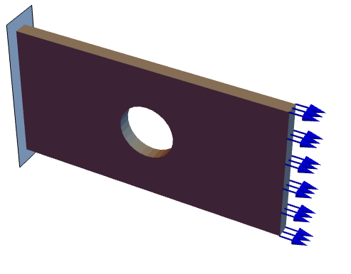
The following test cases verify a 3D stress analysis. The model domain is a perforated plate with a length of , a width of , a height of . The perforation is at center and has a diameter of . At the left boundary the plate is fixed to a wall. At the right hand side a force of is acting in the direction. The remaining boundaries are free to move. As a material a S235 steel is used. Thus Young's modulus is given as and Poisson's ratio is .

Test Reference:

M. Brand, Grundlagen FEM mit Solidworks, Vieweg+Teuber, 2011, ISBN: 978-3-8348-1306-0, Page 13

Equation:

The standard stress model is used.

Define the model variables and parameters:

Set up a 3D steady-state solid mechanics model:

Set up a second 3D steady-state solid mechanics model that uses stress and strain functions:

Solution:

An expected maximum von Mises stress of is given.

The analytical estimation of the von Mises stress is given by

where is stress concentration factor from a look up table. In this case the aspect ratio of the radius of the diameter and half the plate's height result in

The nominal stress on the cross section through the perforation is computed to be

The expected maximal stress is then

Specify the reference values:

Boundary Conditions:

The structure is held fixed at the left hand side.

Fix the structure at the left hand side:

On the right hand side a force of acts in the direction.

Set up a boundary load acting to the right:

The remaining sides are free to move.

Region:

Set up the model region and meshes with hexahedron and tetrahedron elements:

Visualize the mesh:

Solve the PDE model and monitor time/memory usage:

Compute strain, the stress and the von Mises stress:

Solve the PDE model and monitor time/memory usage:

Compute strain, the stress and the von Mises stress:

Test 1:

Test the first PDE on the first mesh:

Test 2:

Test the second PDE on the first mesh:

Visualization:

Visualize the von Mises stress:

SolidMechanics-FEM-Stationary-3D-0003

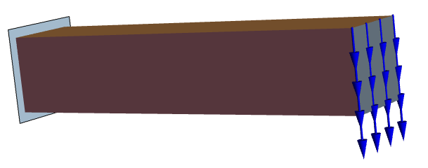
The following test cases verify an applied boundary load. The model domain is a beam with a length of , a width of , a height of . At the left boundary the plate is fixed to a wall. At the right hand side a force of is acting in the negative direction. The remaining boundaries are free to move. As a material a S275 steel is used. Thus Young's modulus is given as and Poisson's ratio is .

Test Reference:

M. Brand, Grundlagen FEM mit Solidworks, Vieweg+Teuber, 2011, ISBN: 978-3-8348-1306-0, Page 29

Equation:

The standard stress model is used.

Define the model variables and parameters:

Set up a 3D steady-state solid mechanics model:

Set up a second 3D steady-state solid mechanics model that uses stress and strain functions:

Solution:

An expected maximum displacement in the negative z direction of is given.

The analytical estimation of the maximum deflection in the direction is given by

where the moment . is the applied force and the length of the beam.

Specify the reference values:

Boundary Conditions:

The structure is held fixed at the left hand side.

Fix the structure at the left hand side:

On the right hand side a force of acts in the negative direction.

Set up a boundary load acting on the right in a downward direction:

The remaining sides are free to move.

Region:

Set up the model region and meshes with hexahedron and tetrahedron elements:

Visualize the mesh:

Solve the PDE model and monitor time/memory usage:

Test 1:

Test the first PDE on the first mesh:

Test 2:

Test the second PDE on the first mesh:

Test 3:

Test the first PDE on the second mesh:

Test 4:

Test the second PDE on the second mesh:

Comment:

The example goes further and computes a normal stress at the fixation of the beam and the wall. The numerical value deviates from the analytical solution because of stress singularities. In the given reference a somewhat arbitrary point is chosen for the comparison of the analytical stress value with the numerically computed value close to the singularity. This approach does not seem optimal, so this test will be skipped.

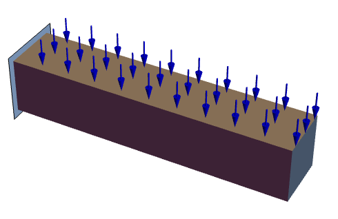
SolidMechanics-FEM-Stationary-3D-0004

The following test cases verify a distributed load. The model domain is a beam with a length of , a width of , a height of . At the left boundary the beam is fixed to a wall. On the top face a load of is applied and acting in the negative direction. Note the units of force per length. The remaining boundaries are free to move. As a material a S275 steel is used. Thus Young's modulus is given as and Poisson's ratio is .

Test Reference:

M. Brand, Grundlagen FEM mit Solidworks, Vieweg+Teuber, 2011, ISBN: 978-3-8348-1306-0, Page 32

Equation:

The standard stress model is used. Note that the material parameters are given in the scale of milli meters .

Define the model variables and parameters:

Set up a 3D steady-state solid mechanics model:

Set up a second 3D steady-state solid mechanics model that uses stress and strain functions:

Solution:

An expected maximum displacement in the negative z direction of is given.

The analytical estimation of the maximum deflection in the direction is given by

where the moment . is the applied distributed force and the length of the beam.

Specify the reference values:

Boundary Conditions:

The structure is held fixed at the left hand side.

Fix the structure at the left hand side:

On the top side a distributed force of acts in the negative direction. Since the length of the beam is the total force acting is .

Set up a boundary load acting on the top:

The remaining sides are free to move.

Region:

Set up the model region and meshes with hexahedron and tetrahedron elements:

Visualize the mesh:

Solve the PDE model and monitor time/memory usage:

Test 1:

Test the first PDE on the first mesh:

Test 2:

Test the second PDE on the first mesh:

Test 3:

Test the first PDE on the second mesh:

Test 4:

Test the second PDE on the second mesh:

Comment:

SolidMechanics-FEM-Stationary-3D-0005

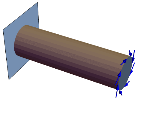
The following test cases verify a torque boundary load. The model domain is a rod with a length of and a diameter of . At the left boundary the rod is fixed to a wall. At the right end a moment of is applied. The remaining boundaries are free to move. As a material a S275 steel is used. Thus Young's modulus is given as and Poisson's ratio is .

Test Reference:

M. Brand, Grundlagen FEM mit Solidworks, Vieweg+Teuber, 2011, ISBN: 978-3-8348-1306-0, Page 35

Equation:

The standard stress model is used.

Define the model variables and parameters:

Set up a 3D steady-state solid mechanics model:

Set up a second 3D steady-state solid mechanics model that uses stress and strain functions:

Solution:

Specify the reference values:

Boundary Conditions:

The structure is held fixed at the left hand side.

Fix the structure at the left hand side:

On the right hand side a torque of is present. This torque needs to be converted into a surface pressure. Starting from

where is the shear stress (a pressure), the radius and the second moment of area [m^4]. After rearranging:

Set up a boundary load acting on the right:

The remaining sides are free to move.

Region:

Set up the model region and create a coarse mesh:

Visualize the mesh:

Solve the PDE model and monitor time/memory usage:

Test 1:

Test the first PDE:

Test 2:

Test the second PDE:

Test 3:

Verify the maximal von Mises stress.

Test 4:

Test the second PDE on the second mesh:

SolidMechanics-FEM-Stationary-3D-0006

A tapered aluminium alloy bar of square cross-section and length is fixated to the ground. An axial load is applied to the free end of the bar.

Test Reference:

C. O. Harris, Introduction to Stress Analysis, The Macmillan Co., New York, NY, 1959, pg. 237, problem 4.

Equation:

The standard stress model is used.

Define the model variables and parameters:

Set up a 3D steady-state solid mechanics model:

Set up a second 3D steady-state solid mechanics model that uses stress and strain functions:

Specify the reference values:

Boundary Conditions:

The bar is fixed at the bottom.

Fix the bar at the bottom (z = 0) and apply a force:

Region:

Set up the model region:

Visualize the mesh:

Solve:

Solve the first PDE model and monitor time/memory usage:

Solve the second PDE model and monitor time/memory usage:

Test 1:

Test the first solution:

Test 2:

Test the second solution:

Test 3:

Test the first solution of the second PDE:

Test 4:

Test the second solution of the second PDE:

Eigenmode Analysis Tests

2D Equations

This section contains examples of 2D eigenmode solid mechanics PDE analysis.

SolidMechanics-FEM-Stationary-2D-Eigenmode-0001

The following test case verifies a 2D plane stress analysis of a beam. The model domain is a beam with a total length of , a height of and thickness . At the left boundary the beam is fixated to a wall. The remaining boundaries are free to move. Young's modulus is given as and Poisson's ratio is . The mass density is given as .

Test Reference:

None

Equation:

The standard stress model is used.

Define the model variables and parameters:

Set up a 2D steady-state solid mechanics model:

Solution:

The expected natural frequencies be computed with:

Here is Youngs modulus, the height, the width, the mass density, the beam length and is:

It follows that

Specify the reference values:

Boundary Conditions:

The beam is fixed at the left hand side.

Fix the structure at the left hand side:

Region:

Set up the model region:

Visualize the mesh:

Solve:

Solve the PDE model and monitor time/memory usage:

Test 1:

Test the first solution:

Test 2:

Test the second solution:

Visualization:

Visualize the deformed structure:

3D Equations

This section contains examples of 3D eigenmode solid mechanics PDE analysis.

SolidMechanics-FEM-Eigenmode-3D-0001

The following test cases verify a 3D eigen mode analysis. The model domain is a beam with a length of , a width of , a height of . At the left boundary the beam is fixed to a wall. The remaining boundaries are free to move. Young's modulus is given as and Poisson's ratio is . The mass density is .

Test Reference:

None

Equation:

The standard stress model is used.

Define the model variables and parameters:

Set up a 3D steady-state solid mechanics model:

Solution:

The expected natural frequencies be computed with:

Here is Youngs modulus, the moment of inertia, the mass density, the area of the cross section and the beam length. The is a factor dependent on the vibration mode and given as

It follows that

Specify the reference values:

Boundary Conditions:

The structure is held fixed at the left hand side.

Fix the structure at the left hand side:

The remaining sides are free to move.

Region:

Set up the model region and meshes with hexahedron and tetrahedron elements.

Visualize the mesh:

Solve the PDE model and monitor time/memory usage:

Test 1:

Test the first solution:

Test 2:

Test the second solution:

Visualization:

Visualize the deformed structure:

SolidMechanics-FEM-Eigenmode-3D-0002

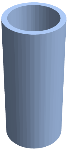
The following test cases verify a 3D eigen mode analysis. The model domain is a cylinder with a height of , an internal radius of , an external radius of . The cylinder is free to move. Young's modulus is given as and Poisson's ratio is . The mass density is .