Solid Mechanics
| Contents | Solid Mechanics Boundary Conditions |
| Introduction | Appendix |
| Overview Example and Analysis Types | Nomenclature |
| Equations | References |
Contents
Introduction
The analysis and behavior of solids under loads and constraints is of fundamental importance in mechanics. Solid mechanics deals with the mechanics of solid bodies in three dimensions, while the topic of structural mechanics encompasses a wider range of objects, such as thin shells or beams, for example.
This tutorial gives an introduction to modeling solid mechanics with partial differential equations. Equations and boundary conditions that are relevant for performing solid mechanics analysis are derived and explained.
Modeling solid mechanics with partial differential equations (PDEs) is not the only way to model solid mechanics. Other techniques include setting up ordinary differential equations (ODEs). This approach is followed by the Wolfram System Modeler. Roughly speaking, the system modeler approach is more suitable for large systems of solid bodies interacting, while the partial differential equation approach is more suitable for a fine-grained analysis of a specific body. In some cases, it is beneficial to use a combination of the two approaches.
The approach taken here is that in an introductory section, a single solid body, a bookshelf bracket, is used to introduce various solid mechanics analysis types and the functionality available. This will be followed by a more theoretical explanation of the underlying ideas and concepts. The theoretical background is much easier to understand once an intuition for the various analysis types exists. After that, the available boundary conditions are discussed.
Solid mechanics typically considers three-dimensional solid objects. Special cases exist to deal with two-dimensional simplifications. These simplifications, however, have some pitfalls that are avoidable if the understanding for the three-dimensional scenario is correct. For this reason, the initial examples will be three-dimensional examples. At a later stage, plane (two-dimensional) stress and strain and their limitations will be introduced.
The goal of a solid mechanics analysis is to find the deformation of a body under load. A subsequent step then finds strains and stresses within the deformed body. The analysis and interpretation of these physical quantities are useful to create a better quality engineering design of the body under consideration. For example, structurally weak parts of an object can be identified and improved upon.
The solid mechanics analysis process is typically done in stages. First, for the body to be analyzed, a geometric model needs to be created. The geometric model is typically created within a computer-aided design (CAD) process. CAD models can either be imported or created in product. To import geometries, common file formats like DXF, STL or STEP are supported. These geometries can be imported with Import. The alternative is to create the geometrical models in product, for example, by using OpenCascadeLink. Once the geometric model is made available, some thought needs to be put into what type of analysis is to be performed. Currently supported analysis types are static analysis, time-dependent analysis, eigenmode analysis and frequency response analysis. The next step is the setup of boundary conditions and constraints. Materials to be used further specify the PDE model. Once the PDE model is fully specified, the subsequent finite element analysis will then compute the desired quantities of the body under investigation. These quantities are then post-processed, either by visualizing them or some derived quantities are computed. This tutorial shows the necessary steps for everything except the CAD model generation.
The modeling process as such results in a system of partial differential equations (PDEs) that can be solved with NDSolve, ParametricNDSolve and NDEigensystem.
The accuracy and the effectiveness of the solid mechanics PDE model is validated in the separate documentation entitled Solid Mechanics Model Verification Tests.
Many of the animations of the simulation results shown here are generated with a call to Rasterize. This is to reduce the disk space required. The downside is that the visual quality of the animations will not be as crisp as without it. To obtain high-quality graphics, remove or comment out the call to Rasterize.
(*frames=Rasterize[#1,"Image",ImageResolution->35]&/@frames;*)The symbols and corresponding units used throughout this tutorial are summarized in the Nomenclature section.
Overview Example and Analysis Types
To illustrate the usage of the finite element method in solid mechanics, it is instructive to present a simple example and give an overview of the setup, various analysis types and post-processing steps possible.
Needs["NDSolve`FEM`"]
$HistoryLength = 0;
The first example introduces the workflow of setting up a simple solid mechanics PDE model. Subsequent sections will then use more sophisticated and complete models. For now, consider the following setup with a long beam fixed at the left and with a downward force applied at the right side.

Creating a solid mechanics model always comprises the same steps:
Ω = Cuboid[{0, 0, 0}, {10, 1, 1}];vars = {{u[x, y, z], v[x, y, z], w[x, y, z]}, {x, y, z}};The dependent variables ![]() ,
, ![]() and
and ![]() represent the displacement in the
represent the displacement in the ![]() ,
, ![]() and
and ![]() directions, respectively.
directions, respectively.
pars = <|"Material" -> Entity["Element", "Titanium"]|>;Subscript[Γ, force] = SolidBoundaryLoadValue[x == 10, vars, pars, <|"Force" -> {0, 0, Quantity[-1000, "Newtons"]}|>];
Subscript[Γ, wall] = SolidFixedCondition[x == 0, vars, pars];MatrixForm[op = SolidMechanicsPDEComponent[vars, pars]]The output has been abbreviated since it is large and hard to read, but this is why using the PDEModel components is convenient.
beamDisplacement = NDSolveValue[{op == Subscript[Γ, force], Subscript[Γ, wall]}, {u[x, y, z], v[x, y, z], w[x, y, z]}, {x, y, z}∈Ω];In many cases like this there is no need to generate a mesh; passing the geometry to the solver is sufficient.
VectorDisplacementPlot3D[beamDisplacement, {x, y, z}∈Ω, PlotLegends -> Automatic]VectorDisplacementPlot3D will automatically rescale the deformation to make it visible. The actual, very small deformation can be seen by specifying the option VectorSizes Full. For this reason it is useful to plot a legend that quantifies the displacement.
This gives an overview of the workflow. The next sections describe the steps in more detail on a more elaborate geometric model.
Geometry
For the following overview of available solid mechanics analysis types, a predefined boundary element mesh is loaded. For more information on how this boundary element mesh was generated, refer to the Bookshelf Bracket tutorial, which explains the creation of this specific geometric model.
bmesh = Import[FileNameJoin[{$InstallationDirectory, "SystemFiles", "Components", "PDEModels", "SupportFiles", "BookShelfBracket.wxf"}]]edgeframe = bmesh["Edgeframe"];
outline = Show[edgeframe, bmesh["Wireframe"["MeshElementStyle" ->
Directive[Opacity[0.2], FaceForm[LightBlue], EdgeForm[]]]]
]Sometimes it is useful to check the imported boundary mesh for defects. If defects are found, a legend with the defects will be displayed. In this case, no defects are found.
FindMeshDefects[MeshRegion[bmesh]]One thing to keep in mind is the scale used in the geometric model. If the length of the boundary mesh is, for example, in units of meters, then the material parameters will need to be specified in consistent units. In this specific case, the units of the boundary mesh are in meters, so the bracket is 0.2 meters long.
The amount of detail of the geometry will affect the number of elements a finite element mesh will need to represent that geometry. The number of elements in a mesh has a direct influence on the CPU time and memory needed to solve a particular problem. To reduce the number of elements, one can consider that geometric details, such as the screw holes, often only have an influence in their closer surroundings [11, c.1]. Saint Venant's principle suggests that a detail with a characteristic length ![]() will affect the surroundings in a distance of about
will affect the surroundings in a distance of about ![]() . If one is interested in the mechanical performance of the object in a specific region that is far enough away from a particular detail, that detail might be left out of the geometric model and thus save computational effort. Also for vibration analysis, geometric details that are smaller than about 10% of the geometric cross section can usually be neglected.
. If one is interested in the mechanical performance of the object in a specific region that is far enough away from a particular detail, that detail might be left out of the geometric model and thus save computational effort. Also for vibration analysis, geometric details that are smaller than about 10% of the geometric cross section can usually be neglected.
In this case, the bracket geometry does not have a screw thread. This will be taken care of when specifying the boundary conditions.
Generally speaking, one should start with as simple a geometric model as possible and only add details to see if and how they affect the overall solution.
More information on generating or importing 3D geometric models can be found in the Using OpenCascadeLink tutorial.
Material Parameters
The next step is to assign material parameters. Generally, all parameters for a solid mechanics model are collected in an Association pars that includes the necessary parameter values.
<|"YoungModulus" -> 210 * 10 ^ 9, "PoissonRatio" -> 0.3, "MassDensity" -> 7850, "ThermalExpansion" -> 8.6 * 10 ^ -6|>;A more convenient way to do material parameter setup is to select a material from an Entity. A convenient way to get to an Entity is it make use of the free-form input for WolframAlpha.
pars = <|"Material" -> Entity["Element", "Titanium"]|>;Material parameters where the values are given as Quantity objects can be used. Should a material not be available or different units be needed, then the material properties can be added by specifying parameters like YoungModulus and PoissonRatio directly. The exact property names needed can be found on the reference page of SolidMechanicsPDEComponent.
The default material model is a linear elastic isotropic material. As a rule of thumb, a linear elastic material model is applicable until a maximal stretching of 5% is reached [8, p. 159].
Geometries consisting of several materials can also be used, and an example of such a use case is presented in the section on multiple materials.
Units
Should the units of the geometry be different from the material units, then the material units can be scaled.
<|"Material" -> Entity["Element", "Titanium"], "ScaleUnits" -> {"Meters" -> "Millimeters"}|>;Internally, all material data units are converted to "SIBase" units. As a consequence, the default unit of length is "Meters". If the units of the geometry are also in meters, then nothing needs to be changed. If the units of the geometry are not in meters, then either the PDE and material properties need to be scaled to the units the geometry or the geometry needs to be scaled to "Meters". To scale the units of the PDE and material parameters, the parameter "ScaleUnits" can be given. If not explicitly stated otherwise, examples in this tutorial use the default "SIBase" units.
Boundary Conditions
Since solid mechanics is about the deformation of objects under load and constraints, boundary conditions are an essential component of solid mechanics modeling. A boundary load is a force or pressure that is applied on the surface of an object. For a load to be applicable to an object, that object must also be constrained in some way, for example, screwed to a wall, as otherwise the object would not pose a resistance to the load. Loads and constraints are set up by specifying boundary conditions. Various boundary conditions can be used and will be discussed in more detail in the boundary conditions section. For the purpose of this overview, a boundary surface load and the constraints introduced by a wall and screws will be sufficient.
The purpose of this section is to establish the positions where the boundary conditions are to be applied. The positions of boundary conditions applied will remain the same, regardless of the analysis type performed. The exact specification of the values of the boundary conditions, however, depends on the different analysis types and will follow in the respective sections.
A way to find the positions where the boundary conditions apply is to visualize them together with the outline of the geometry defined previously in the geometry section.
boundaryLoadPosition = x >= 0.01 && z == 0.19;Show[outline, Graphics3D[{...}], Region[Style[ImplicitRegion[boundaryLoadPosition, {{x, -0.01, 0.2}, {y, 0, 0.05}, {z, 0, 0.2}}], Red]]]SolidBoundaryLoadValue[boundaryLoadPosition, vars, pars, <|"Force" -> {Subscript[f, x], Subscript[f, y], Subscript[f, z]}|>];In a next step, a constraint is added to specify that the bracket is mounted to a wall. To fix the bracket to the wall, two constraints play a role. First, the back of the bracket cannot penetrate the wall and second, screws fix the bracket to the wall.
The screws impose a constraint such that the movement of the surfaces that make the screw hole is prohibited in all directions. This means at the points of contact of the screw and the bracket, no movement is possible at all.
The bracket cannot penetrate the wall, and thus a constraint of the movement of the back of the bracket in the negative ![]() direction is added. Because the two screws press the bracket to the wall and the bracket cannot bend into the wall, a reasonable approach is to also limit the movement in the positive
direction is added. Because the two screws press the bracket to the wall and the bracket cannot bend into the wall, a reasonable approach is to also limit the movement in the positive ![]() (out from the wall) direction. This is a common simplification. If this simplification is not justified, then a contact problem arises.
(out from the wall) direction. This is a common simplification. If this simplification is not justified, then a contact problem arises.
backConstraintPosition = x == 0;Show[outline, Graphics3D[{...}],
Region[Style[ImplicitRegion[backConstraintPosition, {{x, -0.01, 0.2}, {y, 0, 0.05}, {z, 0, 0.2}}], Red]]]SolidDisplacementCondition[backConstraintPosition, vars, pars, <|"Displacement" -> {0, None, None}|>];Next, the constraint for the screws is described.
screwConstraintPosition = ((y - 0.025) ^ 2 + (z - 0.05) ^ 2 <= (0.01) ^ 2) || ((y - 0.025) ^ 2 + (z - 0.15) ^ 2 <= (0.01) ^ 2);Two large enough cylindrical regions are used to cover the screw holes and chamfer.
Show[outline, Graphics3D[{...}],
	Region[Style[ImplicitRegion[screwConstraintPosition, {{x, -0.01, 0.02}, {y, 0, 0.05}, {z, 0, 0.2}}], Red]]
]SolidFixedCondition[screwConstraintPosition, vars, pars];For more complicated geometries, a different technique to specify boundary condition predicates may be appropriate and is given in the appendix in the section Boundary Condition Predicates.
Mesh Generation
To perform a finite element analysis, the boundary mesh representation of the geometric model needs to be discretized into a mesh.
mesh = ToElementMesh[bmesh]More information about the mesh generation process can be found in the Element Mesh generation tutorial. Another option is to import a mesh. Some common mesh file formats can be imported with the help of the FEMAddOns.
Stationary Analysis
A solid mechanics analysis will seek the displacement of an object, which is a consequence of applied forces and constraints. The dependent variables for the displacement are called ![]() ,
, ![]() and
and ![]() and represent the displacements in the
and represent the displacements in the ![]() ,
, ![]() and
and ![]() axis directions, respectively.
axis directions, respectively.
vars = {{u[x, y, z], v[x, y, z], w[x, y, z]}, {x, y, z}};op = SolidMechanicsPDEComponent[vars, pars];The default setup generates a model for a linear elastic isotropic material with a small deformation assumption. This model does not include the self-weight of the object. This can be added with the parameter "BodyLoadValue". Adding that is explained in the section Body Load.
Subscript[Γ, load] = SolidBoundaryLoadValue[boundaryLoadPosition, vars, pars, <|"Force" -> {0, 0, -500}|>];Subscript[Γ, back] = SolidDisplacementCondition[backConstraintPosition, vars, pars, <|"Displacement" -> {0, None, None}|>];Subscript[Γ, screws] = SolidFixedCondition[screwConstraintPosition, vars, pars];AbsoluteTiming[displacement = NDSolveValue[{op == Subscript[Γ, load], Subscript[Γ, screws], Subscript[Γ, back]}, {u[x, y, z], v[x, y, z], w[x, y, z]}, {x, y, z}∈mesh];]The result is a list of three InterpolatingFunction objects. Each InterpolatingFunction gives the displacement for its respective dependent variable. The three InterpolatingFunction objects make up the displacement vector.
More information about the solution process and its options can be found in the NDSolve Options for Finite Elements tutorial.
Post-processing
The primary solution of a solid mechanics PDE model is the displacement that results due to the acting forces. This displacement can be used to visualize how the body deforms under the load and constraints. Also of interest are, however, the stresses and strains in the object. The strains in the body are recovered from the displacement. The stresses are then recovered from the strains. So both the strain and stress are secondary unknowns. The recovered strains and stresses can furthermore be combined in overview concepts like the equivalent strain or the von Mises stress. The terminology post-processing is an umbrella term for all computations and visualizations done after the displacements have been computed.
Deformations
The displacements are often termed ![]() ,
, ![]() and
and ![]() and are the computed displacements in the
and are the computed displacements in the ![]() ,
, ![]() and
and ![]() directions, respectively. Sometimes a displacement vector
directions, respectively. Sometimes a displacement vector ![]() is used.
is used.
The deformation of an object under load is simply the computed displacement added to the coordinates of the original object. A point ![]() in an object originally at
in an object originally at ![]() is moved to
is moved to ![]() when the object is under load.
when the object is under load.
deformedMesh = ElementMeshDeformation[mesh, displacement]Show[mesh["Edgeframe"], deformedMesh["Edgeframe"],
deformedMesh["Wireframe"[
"ElementMeshDirective" -> Directive[EdgeForm[], FaceForm[LightGray]]]]]The deformation shown is scaled by the minimal size of the geometries' extension and the maximal displacement. This can be switched off or changed by specifying a "ScalingFactor" for ElementMeshDeformation. For more information, see the Element Mesh Visualization tutorial.
Show[mesh["Edgeframe"],
	ElementMeshDeformation[mesh, displacement, "ScalingFactor" -> 10]["Wireframe"[
	"ElementMeshDirective" -> Directive[EdgeForm[], FaceForm[LightGray]]]]]
ElementMeshDeformation by default will make the deformation visible, regardless how small it is, as long as it is nonzero; however, the visualization does not depict the true deformation. The true deformation can be shown by setting "ScalingFactor"->None.
Show[mesh["Edgeframe"],
	ElementMeshDeformation[mesh, displacement, "ScalingFactor" -> None]["Wireframe"[
	"ElementMeshDirective" -> Directive[EdgeForm[], FaceForm[LightGray]]]]]
In most cases, deformations are small, and so "ScalingFactor"->None will not give an interesting plot.
Another consequence of the automatic scaling factor computation is that if the body load is increased, the deformation plot will remain the same, as the values will be scaled back again. The value of the deformation plot is in seeing how the body deforms. This can give an idea if the model works as expected.
Sometimes it is useful to know the value of the automatic scaling factor computed.
maxDeformation = Max[Abs[Subtract@@@(MinMax /@ (#["ValuesOnGrid"]& /@ displacement[[All, 0]]))]];
minSize = Min[Abs[Subtract@@@(MinMax /@ Transpose[mesh["Coordinates"]])]];
minSize / maxDeformationInspecting the total displacement is a way to get an overview of the displacement of a constrained object under load. The total displacement is given by:
where ![]() ,
, ![]() and
and ![]() are the computed displacements in the
are the computed displacements in the ![]() ,
, ![]() and
and ![]() directions, respectively.
directions, respectively.
SliceContourPlot3D[Sqrt[Total[displacement ^ 2]], mesh, {x, y, z}∈mesh, ColorFunction -> "Temperature", PlotLegends -> Automatic]Strains
Strain is a quantity that describes the amount of deformation within a body [2] and is a ratio and unitless. Strain is not to be confused with the amount of displacement. Strain is related to the displacement by the gradient of a given displacement. The concept of strain will be explained in more detail in the theory section about strain.
strains = SolidMechanicsStrain[vars, pars, displacement]The SolidMechanicsStrain function computes the normal and shear strains for each independent direction. The function returns a SymmetrizedArray that contains an expression representing the strain components in the various directions. The SymmetrizedArray enforces symmetry when present and is compact. The strains returned have the following order:

where the normal strains are denoted by ![]() and the shear strains by
and the shear strains by ![]() . The software uses engineering strains by default and
. The software uses engineering strains by default and ![]() . It is possible to switch off the usage of engineering strains by setting "EngineeringStrain"->False in the parameters pars. This may be of interest when comparing linear material laws with nonlinear material laws, where true stain is used. More information can be found in the reference page of SolidMechanicsStrain.
. It is possible to switch off the usage of engineering strains by setting "EngineeringStrain"->False in the parameters pars. This may be of interest when comparing linear material laws with nonlinear material laws, where true stain is used. More information can be found in the reference page of SolidMechanicsStrain.
Loosely speaking, strain is the gradient of the displacement. Strain plots show where the gradient of displacement is large, not where there is much deformation.
Show[
	mesh["Edgeframe"],
	SliceContourPlot3D[#, mesh, {x, y, z}∈mesh, ColorFunction -> "TemperatureMap", PlotLegends -> Automatic]
	]& /@ Extract[strains, {{1, 1}, {3, 3}}]
Note in this example the absolute values of the strain in the ![]() direction are smaller than absolute values in the
direction are smaller than absolute values in the ![]() direction, even though the displacement in the negative
direction, even though the displacement in the negative ![]() direction is much larger than in the positive
direction is much larger than in the positive ![]() direction.
direction.
MatrixForm[Normal[strains] /. {x -> 0.01, y -> 0.025, z -> 0.19}]Sometime it is useful to visualize the strain results with the same color scale. The minimum and maximum of all strain values are extracted and used to set the bounds for the color scale.
{minStrain, maxStrain} = MinMax[#["ValuesOnGrid"]& /@ Flatten[Normal[strains]][[All, 0]]]Show[
mesh["Edgeframe"],
SliceContourPlot3D[#, mesh, {x, y, z}∈mesh, ColorFunction -> (ColorData["TemperatureMap"][Rescale[#, {minStrain, maxStrain}]]&),
ColorFunctionScaling -> False, PlotLegends -> Automatic]
]& /@ Extract[strains, {{1, 1}, {3, 3}}]Show[
mesh["Edgeframe"],
SliceContourPlot3D[strains[[1, 3]], mesh, {x, y, z}∈mesh, ColorFunction -> (ColorData["TemperatureMap"][Rescale[#, {minStrain, maxStrain}]]&),
ColorFunctionScaling -> False, PlotLegends -> Automatic]
]Sometimes one would like to identify the regions where strains are larger than a specific value.
With[{rmf = ElementMeshRegionMember[mesh, #]&}, Show[mesh["Edgeframe"], RegionPlot3D[Evaluate[(strains[[1, 1]] > 0) && rmf[{x, y, z}]], {x, 0, 0.2}, {y, 0, 0.05}, {z, 0, 0.2}]]]Inspecting all strain components can be cumbersome. The equivalent strain is a simplification that combines all strain components into a scalar, and as such is easier to grasp. However, the equivalent strain does not include the complete picture of the strains.
The equivalent strain computes:
Some implementations of the equivalent strain use a factor of ![]() , where
, where ![]() is Poisson's ratio. This factor has been excluded to ensure the equivalent strain is compatible with the von Mises stress, which is the stress analog of the equivalent strain.
is Poisson's ratio. This factor has been excluded to ensure the equivalent strain is compatible with the von Mises stress, which is the stress analog of the equivalent strain.
equivalentStrain = EquivalentStrain[vars, pars, strains]Show[mesh["Edgeframe"],
SliceContourPlot3D[equivalentStrain, mesh, {x, y, z}∈mesh, ColorFunction -> "TemperatureMap", PlotLegends -> Automatic]]Sometimes it is more convenient to plot the strain over the deformed body.
equivalentStrainFunction = Head[equivalentStrain]deformedEquivalentStrain = ElementMeshInterpolation[deformedMesh, equivalentStrainFunction["ValuesOnGrid"]];Show[mesh["Edgeframe"],
deformedMesh["Edgeframe"],
SliceContourPlot3D[deformedEquivalentStrain[x, y, z], deformedMesh, {x, y, z}∈deformedMesh, ...]]Principal strain values are the main strain values. They are the computed eigenvalues of the strain matrix and correspond to a local coordinate system where the shear strains ![]() are 0. The principal strain values are the
are 0. The principal strain values are the ![]() in the local coordinates and give the load direction independent strains.
in the local coordinates and give the load direction independent strains.
{principalStrainValues, principalStrainVector} = PDEModels`PrincipalEigensystem[vars, pars, strains];Principal strain values are ordered according to their size.
principalStrainValues /. Thread[Rule[{x, y, z}, mesh["Coordinates"][[1]]]]At each evaluation coordinate, there are three principal strains. Each of those principal strains can be interpreted as a vector and visualized.
Show[mesh["Edgeframe"],
VectorPlot3D[principalStrainValues, {x, y, z}∈mesh, VectorPoints -> Fine, PlotLegends -> Automatic, Boxed -> False, Axes -> None]]Show[mesh["Edgeframe"],
VectorPlot3D[principalStrainVector, {x, y, z}∈mesh, Boxed -> False, Axes -> None]]The section Boundary Load: Tension has an example that shows the use of PrincipalEigensystem to find stresses in a nonaxial loaded cylinder.
Stresses
Stress is a quantity that describes the distribution of internal forces within a body [2] and is measured in ![]() or
or ![]() .
.
stresses = SolidMechanicsStress[vars, pars, strains]The Stress function computes the normal stress and shear stress for each independent direction. The function returns a SymmetrizedArray that contains an expression representing the stress component in that direction. The stresses returned have the following order:
where the normal stresses are denoted by ![]() and the shear stresses by
and the shear stresses by ![]() . The first index tells you the direction of the force, while the second index specifies the direction of surface the force is acting on.
. The first index tells you the direction of the force, while the second index specifies the direction of surface the force is acting on.
Show[mesh["Edgeframe"],
	SliceContourPlot3D[#, mesh, {x, y, z}∈mesh, ...]
]& /@ Extract[stresses, {{1, 1}, {3, 3}}]Show[mesh["Edgeframe"],
SliceContourPlot3D[stresses[[1, 3]], mesh, {x, y, z}∈mesh, ...]]MatrixForm[Normal[stresses] /. {x -> 0.01, y -> 0.025, z -> 0.19}]Inspecting all stress variables can be a cumbersome. A simplification that combines all stress components in a single expression is the von Mises stress. The von Mises stress is a scalar and as such, easier to grasp. However, the von Mises stress does not include the complete picture of the stresses present within a body. The von Mises stress is to the stresses the same as the equivalent strain is for the strains.
The von Mises stress computes:
vonMisesStress = VonMisesStress[vars, pars, stresses]vonMisesStressFunction = Head[vonMisesStress]MinMax[vonMisesStressFunction["ValuesOnGrid"]]vonMisesPlot = Show[mesh["Edgeframe"],
SliceContourPlot3D[vonMisesStress, mesh, {x, y, z}∈mesh, ...]]minMaxValues = MinMax[vonMisesStressFunction["ValuesOnGrid"]];
minMaxPos = Flatten[Position[vonMisesStressFunction["ValuesOnGrid"], #, 1, 1]& /@ minMaxValues];
minMaxPosCoords = mesh["Coordinates"][[minMaxPos]];
Show[vonMisesPlot,
ListPointPlot3D[MapThread[Callout, {minMaxPosCoords, minMaxValues}]]]Sometimes it is more convenient to plot the stresses over the deformed body.
deformedVonMisesStress = ElementMeshInterpolation[deformedMesh, vonMisesStressFunction["ValuesOnGrid"]];Show[mesh["Edgeframe"],
deformedMesh["Edgeframe"],
SliceContourPlot3D[deformedVonMisesStress[x, y, z], deformedMesh, {x, y, z}∈deformedMesh, ...]]With[{rmf = ElementMeshRegionMember[mesh, #]&}, Show[mesh["Edgeframe"], RegionPlot3D[Evaluate[(vonMisesStress > 10 ^ 7) && rmf[{x, y, z}]], {x, 0, 0.2}, {y, 0, 0.05}, {z, 0, 0.2}, PlotPoints -> 31]]]Principal stress values are the main stress values. They are the computed eigenvalues of the stress matrix and correspond to the diagonal stress values ![]() where the shear stresses
where the shear stresses ![]() are 0. The principal stress values give stresses independent of load direction.
are 0. The principal stress values give stresses independent of load direction.
{principalStressValues, principalStressVectors} = PDEModels`PrincipalEigensystem[vars, pars, stresses];Evaluated at a coordinate, ![]() returns a list of three values: the first, second and third principal stress values.
returns a list of three values: the first, second and third principal stress values.
principalStressValues /. Thread[Rule[{x, y, z}, mesh["Coordinates"][[1]]]]Show[mesh["Edgeframe"],
VectorPlot3D[principalStressValues, {x, y, z}∈mesh, ...]]principalStressVectors /. Thread[Rule[{x, y, z}, mesh["Coordinates"][[1]]]]Show[mesh["Edgeframe"],
VectorPlot3D[principalStressVectors, {x, y, z}∈mesh, VectorPoints -> {13, 3, 13}, Boxed -> False, Axes -> None]]A legend is not meaningful here, as an eigenvector multiplied by a scalar is still an eigenvector.
The section Boundary Load: Tension has an example that shows the use of PrincipalEigensystem to find stresses in a nonaxial loaded cylinder.
Since PrincipalEigensystem sorts the eigenvalues from largest to smallest, it cannot be used for a symbolic computation of principal eigenvalues, as sorting of symbolic expressions is not possible.
Safety factor
The factor of safety is a number telling us by how large a factor the maximal resulting stresses are below a stress limit. There are multiple definitions of the factor of safety, abbreviated as FOS. Because the material at hand is a metal, which is ductile and not brittle, the von Mises failure criterion is a reasonable choice. For ductile materials, failure is considered to start at the onset of plastic deformation (while for brittle materials, failure is considered at fracture). For more information, see the section Failure Theory.
The principal eigenvalues of a stressed body are computed to transform the stresses into load direction independent stresses, which then can be used to compute the von Mises stress.
{principalStressValues, principalStressVectors} = PDEModels`PrincipalEigensystem[vars, pars, stresses];The equivalent von Mises stress can be computed with the von Mises stress functions if the shear stresses are set to 0.
mat = SymmetrizedArray[DiagonalMatrix[principalStressValues]];
equivalentVonMisesStress = VonMisesStress[vars, pars, mat]equivalentVonMisesStressFunction = Head[equivalentVonMisesStress]maxEquivalent = Max[equivalentVonMisesStressFunction["ValuesOnGrid"]]For ductile material, plastic deformation starts when the stress reaches the yield strength (for brittle materials, when stress reaches the ultimate strength).
yieldStrength = QuantityMagnitude[pars["Material"]["TensileYieldStrength"], "SIBase"]maxEquivalent > yieldStrengthyieldStrength / maxEquivalentA safety factor below one is problematic. In this case, a linear stress-strain relation is assumed; the maximum equivalent stress may be different if a nonlinear stress-strain relation is used. When a linear material model is used outside its realm of validity, the stresses computed are typically higher than the actual stresses. Nevertheless, finding stresses that are higher than the yield stress is something to be very cautious about.
With[{rmf = ElementMeshRegionMember[mesh, #]&}, Show[mesh["Edgeframe"], RegionPlot3D[Evaluate[((yieldStrength / equivalentVonMisesStress) < 10) && rmf[{x, y, z}]], {x, 0, 0.2}, {y, 0, 0.05}, {z, 0, 0.2}, PlotPoints -> 31]]]Reaction forces
Every object that is constrained and at the same time under load will have reaction forces that balance the sum of the loads. These reaction forces will be at the constrained parts of the body.
data = ProcessPDEEquations[{op == Subscript[Γ, load], Subscript[Γ, back], Subscript[Γ, screws]}, {u[x, y, z], v[x, y, z], w[x, y, z]}, {x, y, z}∈mesh];
{displacements, reactionForces} = PDEModels`ReactionForce[data];
The function PDEModels`ReactionForce returns the displacements just as a normal call to NDSolve would and a second set of InterpolatingFunction instances that are the reaction forces.
Total[#["ValuesOnGrid"]]& /@ reactionForcesThe sum of the reaction forces matches the values of the boundary loads.
Subscript[Γ, load]Show[
mesh["Edgeframe"],
VectorPlot3D[Through[reactionForces[x, y, z]], {x, y, z}∈mesh, PlotLegends -> Automatic, ColorFunction -> "TemperatureMap", VectorScaling -> Automatic]]The shown reaction forces counteract the (not shown) downward force that acts on the bracket.
In the current version, the reaction forces can only be computed for linear stationary solid mechanics models.
Time-Dependent Analysis
A time-dependent analysis will have to be used if some of the PDE model components have time-dependent behavior. A common time-dependent component is time-dependent boundary conditions.
tvars = {{u[t, x, y, z], v[t, x, y, z], w[t, x, y, z]}, t, {x, y, z}};
top = SolidMechanicsPDEComponent[tvars, pars];Subscript[Γ, timeload] = SolidBoundaryLoadValue[boundaryLoadPosition, tvars, pars, <|"Force" -> {0, 0, -Sin[2π t]500}|>];An important numerical aspect of dynamically loading an object is that the load is not applied instantaneously. For one thing, such a model is unphysical and will result in long simulation times.
Subscript[Γ, timescrews] = SolidFixedCondition[screwConstraintPosition, tvars, pars];Subscript[Γ, timeback] = SolidDisplacementCondition[backConstraintPosition, tvars, pars, <|"Displacement" -> {0, None, None}|>];Since the time-dependent solid mechanics equations are second order time dependent, the initial conditions comprise an initial displacement and an initial velocity field. Note that the initial conditions affect the whole body. For example, specifying a nonzero initial displacement means the entire body is displaced by the specified amount at the initial time.
ics = {u[0, x, y, z] == 0, v[0, x, y, z] == 0, w[0, x, y, z] == 0, Derivative[1, 0, 0, 0][u][0, x, y, z] == 0, Derivative[1, 0, 0, 0][v][0, x, y, z] == 0, Derivative[1, 0, 0, 0][w][0, x, y, z] == 0};tEnd = 5;
AbsoluteTiming[
Monitor[MaxMemoryUsed[
transientDisplacement = NDSolveValue[{top == Subscript[Γ, timeload], Subscript[Γ, timescrews], Subscript[Γ, timeback], ics}, {u[t, x, y, z], v[t, x, y, z], w[t, x, y, z]}, {x, y, z}∈mesh
, {t, 0, tEnd}
, EvaluationMonitor :> (monitor = Row[{"t = ", CForm[t]}])]] / 1024. ^ 2
, monitor]]frames = Table[Show[mesh["Edgeframe"], ElementMeshDeformation[{t, mesh}, transientDisplacement, "ScalingFactor" -> 10]["Wireframe"[
"ElementMeshDirective" -> Directive[EdgeForm[], FaceForm[LightGray]]]], Boxed -> True, BoxStyle -> Transparent],
{t, 0, tEnd, tEnd / 25}];
frames = Rasterize[#1, "Image", ImageSize -> Small]& /@ frames;ListAnimate[frames]To monitor the movement of a specific point within the body over time, a query point is set up. The query point can then be traced through time.
queryPoint = {0.19, 0.025, 0.185};
Show[
	mesh["Wireframe"],
Graphics3D[{Red, PointSize[0.04], Point[queryPoint]}]]Plot[transientDisplacement[[3]] /. Thread[Rule[{x, y, z}, queryPoint]], {t, 0, tEnd}]Note that the system is not damped and the amplitude of the displacement remains the same over the cycles.
transientStrain = SolidMechanicsStrain[vars, pars, transientDisplacement];
transientStress = SolidMechanicsStress[vars, pars, transientStrain];
transientVonMisesStress = VonMisesStress[vars, pars, transientStress];frames = Table[Show[mesh["Edgeframe"],
SliceContourPlot3D[transientVonMisesStress, mesh, {x, y, z}∈mesh, ColorFunction :> (ColorData["TemperatureMap"][Rescale[#, {0, 5 * 10 ^ 7}]]&),
ColorFunctionScaling -> False, Contours -> 10, PlotLegends -> Automatic]], {t, 0, tEnd, tEnd / 25}];ListAnimate[frames]A time-dependent analysis can take a long time and require a lot of memory. For this reason, it is important to be able to estimate if an analysis really needs to be transient. The time ![]() it takes for a shear wave to travel though an elastic solid with a characteristic length
it takes for a shear wave to travel though an elastic solid with a characteristic length ![]() is approximately [11, c.1]
is approximately [11, c.1]
where ![]() is the mass density and
is the mass density and ![]() is the shear modulus. Stress values decay to their stationary values in about
is the shear modulus. Stress values decay to their stationary values in about ![]() . Similar considerations can be made for stresses induced by acceleration in rotating objects [11, c.1].
. Similar considerations can be made for stresses induced by acceleration in rotating objects [11, c.1].
Eigenmode Analysis
An eigenmode analysis computes the resonant frequencies of an object. These frequencies are also called natural frequencies. At each of these eigenfrequencies, the object under investigation deforms into a distinct shape called eigenmode. The result of an eigenmode analysis is a list of frequencies and their corresponding modes.
There are multiple reasons to compute eigenfrequencies and eigenmodes; among them are:
- Objects in resonance are a common cause of failure. Knowing these frequencies helps avoid the shapes being exposed to them.
The generalized equations of motion for solid mechanics for a linear elastic material are given as:
where ![]() is the mass matrix,
is the mass matrix, ![]() the damping matrix,
the damping matrix, ![]() the stiffness matrix and
the stiffness matrix and ![]() the load vector.
the load vector. ![]() is the displacement vector of dependent variables
is the displacement vector of dependent variables ![]() ,
, ![]() and
and ![]() .
. ![]() is the derivative of the displacement vector, the velocity vector, and
is the derivative of the displacement vector, the velocity vector, and ![]() the second derivative of the displacement, the acceleration. For vibrational analysis, the damping
the second derivative of the displacement, the acceleration. For vibrational analysis, the damping ![]() is generally ignored [7] and results in:
is generally ignored [7] and results in:
In an eigenfrequency analysis, constraints are considered but loads are not considered, thus ![]() .
.
For an eigenfrequency analysis, one is interested in the solution of an equation of this form:
Here, ![]() is the solid mechanics PDE component operator that provides
is the solid mechanics PDE component operator that provides ![]() and
and ![]() .
. ![]() is the eigenvalue
is the eigenvalue ![]() .
.
eigenmodeOperator = SolidMechanicsPDEComponent[tvars, Join[pars, <|"AnalysisType" -> "Eigenmode"|>]];It is worthwhile noting that contrary to other analysis types, the eigenmode analysis needs to be specified as a parameter. In the other cases, SolidMechanicsPDEComponent can deduce the analysis type from the variable specification. The eigenmode analysis is very similar to the time-dependent setup and cannot be deduced from the variable input alone.
Also note that an eigenmode analysis is set up as a time dependent system and it uses a time dependent variable specification.
tvarsFirst, a contained eigenmode analysis is investigated. This means the body is constrained by boundary conditions. The only conditions relevant for a constrained eigenmode analysis are boundary conditions that result in DirichletCondition where a dependent variable is set to 0. Boundary forces and nonzero SolidDisplacementCondition are not relevant.
{evals, evecs} = NDEigensystem[{eigenmodeOperator == {0, 0, 0}, Subscript[Γ, timescrews], Subscript[Γ, timeback]}, tvars[[1]], t, {x, y, z}∈mesh, 6];The eigenvalues ![]() are related to the angular frequencies
are related to the angular frequencies ![]() by:
by:
The angular frequency is related to the frequency ![]() measured in
measured in ![]() by:
by:
The natural frequencies can be computed from the eigenvalues by:
eigenfrequencies = Sqrt[evals] / (2π)GraphicsGrid[Partition[MapThread[Show[
mesh["Edgeframe"[PlotLabel -> Style["freq=" <> ToString[#1] <> " Hz", 8]]],
deformedMesh2 = ElementMeshDeformation[mesh, #2];
deformedMesh2["Edgeframe"],
deformedMesh2["Wireframe"[
"ElementMeshDirective" -> Directive[EdgeForm[], FaceForm[LightGray]]]]
]&, {eigenfrequencies, evecs}], 3]]The amount of the deformation in the deformed shapes is not actual deformations. Keep in mind that the amplitude for the deformations shown is arbitrary. Any constant times an eigenmode is still the same eigenmode. An eigenmode analysis computes the eigenfrequency and the qualitative shape of the modes at the respective frequencies.
A special situation occurs when there are no constraints on the object. Then the first modes will be zero and are called rigid body modes. A rigid body mode represents a body that translates or rotates without deformations. Eigenvalues and modes capture the fundamental shape of deformations a body is capable of. A zero eigenmode accounts for the fact that the body could translate or rotate. The fact that a body can translate or rotate is not news, and thus these modes are of no interest. In three dimensions, there are six rigid body modes, three for the translation in each direction and three for a rotation around each axis.
{evals, evecs} = NDEigensystem[{eigenmodeOperator == {0, 0, 0}}, tvars[[1]], t, {x, y, z}∈mesh, 12];eigenfrequenciesUnconstraint = Re[Sqrt[evals] / (2π)]Note that the first six eigenvalues are relatively close to 0 and represent the rigid body modes. Also note that rigid body modes can have eigenvalues with small imaginary parts.
GraphicsGrid[Partition[MapThread[Show[
	mesh["Edgeframe"],
	deformedMesh2 = ElementMeshDeformation[mesh, #2];
	deformedMesh2["Edgeframe"],
	deformedMesh2["Wireframe"[
	"ElementMeshDirective" -> Directive[EdgeForm[], FaceForm[LightGray]]]]
	]&, {eigenfrequenciesUnconstraint, evecs}[[All,  ;; 6]]], 3]]
These are the rigid body modes. A rigid body that is translated or rotated has a zero eigenvalue. All in all, there are three possible translations in the corresponding ![]() ,
, ![]() and
and ![]() axis directions and three rotations around the same axis. The eigenmodes found by the eigensolver are not the pure rigid body modes but are a superposition of combinations of the fundamental rigid body movements.
axis directions and three rotations around the same axis. The eigenmodes found by the eigensolver are not the pure rigid body modes but are a superposition of combinations of the fundamental rigid body movements.
If a modal analysis reveals rigid body modes, then the object is not constrained enough. An eigenanalysis is a good check to verify that the body is sufficiently constrained.
Parametric Analysis
Sometimes one would like to vary a parameter of a PDE model and repetitively solve the same PDE for a variety of parameters. A convenient way to do so is a parametric analysis. In the bookshelf example, it might be of interest how the bookshelf deforms under various surface loads. In this case, the boundary load force is made a parameter. The simulation is set up in exactly the same way as in a nonparametric analysis, only using the ParametricNDSolve family of functions and specifying the name of the parameter in the model.
Subscript[Γ, loadParametric] = SolidBoundaryLoadValue[boundaryLoadPosition, vars, pars, <|"Force" -> {0, 0, -force}|>];pfun = ParametricNDSolveValue[{op == Subscript[Γ, loadParametric], Subscript[Γ, screws], Subscript[Γ, back]}, {u[x, y, z], v[x, y, z], w[x, y, z]}, {x, y, z}∈mesh, {force}]parametricForces = {100, 500, 1000};
displacements = pfun /@ parametricForces;SliceContourPlot3D[Sqrt[Total[# ^ 2]], mesh, {x, y, z}∈mesh, ColorFunction -> "Temperature", PlotLegends -> Automatic]& /@ displacementsNote that the results remain qualitatively the same, but the magnitude of the total displacement changes linearly with the force applied.
Force displacement plot
A parametric analysis can be use to create force-displacement plots. For a specific query point, the displacement is tracked while the force increases.
parametricForces = Range[100, 1000, 100];
displacements = pfun /@ parametricForces;ListLinePlot[Transpose[{Sqrt[Total[(displacements /. {x -> 0.199, y -> 0.025, z -> 0.185}) ^ 2, {2}]], parametricForces}], ...]A linear behavior between force and displacement is observed, which is expected for the linear material model that is used by default.
Parametric material laws
It is possible to have parametric material laws. For example, the Poisson ratio, or a heat transfer coefficient could be parametric. These cases work like any other parametric case. The only thing to be aware of is that material law parameter values need to be respecified when computing the strain and stress.
parametricPars = <|"PoissonRatio" -> ν, "YoungModulus" -> 1|>;
paramerticOp = SolidMechanicsPDEComponent[vars, parametricPars];pfun = ParametricNDSolveValue[{paramerticOp == Subscript[Γ, load], Subscript[Γ, screws], Subscript[Γ, back]}, {u[x, y, z], v[x, y, z], w[x, y, z]}, {x, y, z}∈mesh, {ν}]parametricPoissonRatio = {1 / 10, 3 / 10, 4 / 10};
displacements = pfun /@ parametricPoissonRatio;In this case, the strain computation does not depend on the Poisson ratio parameter ![]() and can be done in the usual way.
and can be done in the usual way.
strains = SolidMechanicsStrain[vars, parametricPars, #]& /@ displacements;The stress computation, however, does depend on the Poisson ratio parameter ![]() . In this case, the parametric parameters need to have the actual parameter value for the computation. This can be done by replacing the symbolic parameter value with the actual value.
. In this case, the parametric parameters need to have the actual parameter value for the computation. This can be done by replacing the symbolic parameter value with the actual value.
stresses = MapThread[SolidMechanicsStress[vars, parametricPars /. ν -> #1, #2]&, {parametricPoissonRatio, strains}]Frequency Response Analysis
A frequency response analysis gives information on how a specific point in a body reacts to a sweep through a frequency range. The result of a frequency response analysis is a frequency response plot showing the relation between real displacement at the range of frequencies. The frequency response analysis is also called harmonic analysis.
Before performing a frequency response analysis, it can be useful to perform an eigenmode and a static analysis. The eigenmode analysis will find the critical frequencies and their related modes that will play a part in the frequency response analysis. The static analysis will provide the maximum displacement without any frequency component.
In the solid mechanics domain, a frequency response analysis in effect solves:
Here ![]() is the angular frequency,
is the angular frequency, ![]() the imaginary init and
the imaginary init and ![]() the resulting displacement.
the resulting displacement. ![]() ,
, ![]() and
and ![]() are the mass, damping and stiffness of the solid mechanics PDE. These are provided by SolidMechanicsPDEComponent.
are the mass, damping and stiffness of the solid mechanics PDE. These are provided by SolidMechanicsPDEComponent.
In this case, like above, the undamped case such that ![]() is considered.
is considered.
fvars = {{u[x, y, z], v[x, y, z], w[x, y, z]}, ω, {x, y, z}};
fop = SolidMechanicsPDEComponent[fvars, pars];
To perform a frequency response analysis, a frequency-dependent load or constraint needs to be set up. This is in contrast to an eigenmode analysis, where boundary loads are not relevant.
Subscript[Γ, frequencyload] = SolidBoundaryLoadValue[boundaryLoadPosition, fvars, pars, <|"Force" -> {0, 0, -Sin[ω]500}|>];The remaining boundary conditions are the stationary boundary conditions.
pfun = ParametricNDSolveValue[{fop == Subscript[Γ, frequencyload], Subscript[Γ, screws], Subscript[Γ, back]}, {u[x, y, z], v[x, y, z], w[x, y, z]}, {x, y, z}∈mesh, ω]Choose a frequency range from the minimal eigenfrequency to the largest eigenfrequency computed.
frequencyList = Table[ 10. ^ i / (2π), { i, 3, 4.5, 0.05}]angularFrequencyList = 2π frequencyList;harmonicSolutions = pfun /@ angularFrequencyList;queryPoint = {0.19, 0.025, 0.185};
Show[
mesh["Edgeframe"],
Graphics3D[{Red, PointSize[0.04], Point[queryPoint]}]]queryPointDisplacement = Sqrt[Total[(harmonicSolutions /. Thread[Rule[{x, y, z}, queryPoint]]) ^ 2, {2}]]ListLogPlot[Transpose[{frequencyList, queryPointDisplacement}], ...]To get a better understanding of the result, frequency responses are compared with the stationary solution. For the frequency response analysis, a frequency-dependent load Subscript[Γ, frequencyload]![]()
![]() in the negative
in the negative ![]() direction is used. In the stationary analysis, a comparable boundary load
direction is used. In the stationary analysis, a comparable boundary load Subscript[Γ, load]![]()
![]() in the negative
in the negative ![]() direction was used. It is interesting to find the displacement of the query point from the stationary solution. This allows putting the frequency response displacements in relation to the displacement of the query point in the stationary solution.
direction was used. It is interesting to find the displacement of the query point from the stationary solution. This allows putting the frequency response displacements in relation to the displacement of the query point in the stationary solution.
staticDisplacement = Sqrt[Total[displacement ^ 2]] /. Thread[Rule[{x, y, z}, queryPoint]]ListLogPlot[{Transpose[{frequencyList, queryPointDisplacement}], {{1, staticDisplacement}, {1.7 3 10 ^ 3, staticDisplacement}}}, ...]Close to the resonance frequency, the maximal displacement of the query point is about one order of magnitude larger than the displacement of that same point in the stationary analysis.
pos = Position[queryPointDisplacement, Max[queryPointDisplacement]];
Extract[frequencyList, pos]
In the previous section, the eigenvalues of the constrained bookshelf were computed.
eigenfrequencies[[1 ;; 6]]Overall, this means that when the body is in resonance, the amount of deformation can be much larger than what is caused by a comparable stationary force.
Note that evaluating the parametric harmonic function at the resonant frequencies computed during the eigenmode analysis may not be possible.
resonantHarmonic = 2π eigenfrequencies[[5]]pfun[resonantHarmonic]Equations
Overview
Solid mechanics is the analysis of bodies under load and constraints. The entire topic of solid mechanics hinges around four components:
These components are related in the following manner:

Before going into too much detail, a broad overview of the different solid mechanics components is shown.
Equilibrium equations
The equilibrium equations relate a force density ![]()
![]() and the stress
and the stress ![]()
![]() . Loosely speaking, stress
. Loosely speaking, stress ![]() is the resistance of an internal point to the applied load. The time-dependent equilibrium equation is given by:
is the resistance of an internal point to the applied load. The time-dependent equilibrium equation is given by:
where ![]() is the mass density and
is the mass density and ![]() the displacement vector. A load
the displacement vector. A load ![]() can either be acting on the entire body or the boundary. To simplify things, the time-dependent term is ignored for now. The component form of the time-independent equilibrium equation
can either be acting on the entire body or the boundary. To simplify things, the time-dependent term is ignored for now. The component form of the time-independent equilibrium equation ![]() in three-dimensional space for the stress components
in three-dimensional space for the stress components ![]() and body forces
and body forces ![]() is given by:
is given by:
Kinematic equations
The kinematic equations relate the displacement ![]() to the strain
to the strain ![]() . Strain
. Strain ![]() describes the relative displacement between points in the body. There are various strain measures. Here, two approaches are distinguished. In the infinitesimal deformation theory, it is assumed that the displacements and strains are small. This is the default method in SolidMechanicsPDEComponent. The infinitesimal strain measure is given by:
describes the relative displacement between points in the body. There are various strain measures. Here, two approaches are distinguished. In the infinitesimal deformation theory, it is assumed that the displacements and strains are small. This is the default method in SolidMechanicsPDEComponent. The infinitesimal strain measure is given by:
For the finite deformation theory, no assumptions are made. If the strain-displacement relation is nonlinear, it is referred to as geometric nonlinearity. The finite deformation theory is such a geometric nonlinearity. Geometric nonlinearity is also called a nonlinear kinematic equation. A geometric nonlinearity accounts for the fact that the geometry is evolving during the loading.
Constitutive equations
The relation of the equilibrium equations—the forces—and the kinematic equations—the description of deformation—is done through the constitutive equations. The constitutive equations, also known as the material model, relate stress to strain. Generally speaking, this is a relationship of the form
where a function ![]() relates the strain and other field quantities to the stress. The most important relation is Hooke's law, where the relation between stress and strain is linear and given by:
relates the strain and other field quantities to the stress. The most important relation is Hooke's law, where the relation between stress and strain is linear and given by:
where the proportionality constant ![]() is the Young's modulus. Most metals and alloys can be modeled as an elastic material if the strains remain small.
is the Young's modulus. Most metals and alloys can be modeled as an elastic material if the strains remain small.
If a linear relation between stress and strain cannot be assumed, a nonlinear constitutive equation is present. This is also referred to as a nonlinear material law.
Besides linearity, there are other properties of interest in a material law. The deformation of an object is called elastic if after removing a force, the object returns to its original configuration. Plastic deformation occurs when the object does not return to its original configuration after the loads are removed. Energy is lost whenever an object experiences plastic deformation. Plastic deformation is permanent. Plasticity is a special form of material nonlinearity.
The current version allows for elastic material models that can be linear or nonlinear. Plasticity is reserved for a future version.
Equilibrium Equations
No material properties (constitutive equations) are used in the derivation of the equilibrium equations and as such, they are applicable to all materials. The equilibrium equation is given by:
The presented solid mechanics formulation is based on displacements as primary unknowns. This is a common approach [4, p.480], as the finite element solver will compute the displacements. The secondary unknowns such as strain and stress will be recovered from the displacements. While it is conceivable that equations are set up in such a manner that all unknowns are solved for, the resulting system of equations will become prohibitively large to solve in a reasonable time and with limited computer memory available.
The units of the solid mechanics model terms are force density in ![]() .
.
Body load
Body loads are forces that act on the entire volume of the object and arise from external force fields. These forces are also called volume forces and are specified as a force density in ![]() . Body loads are often also called body forces, but really they are a force per unit volume. Body loads can be specified with the parameter "BodyLoad" and are specified as a vector field. Gravity is an example of a constant body load; a position-dependent centrifugal force in rotating objects is another example.
. Body loads are often also called body forces, but really they are a force per unit volume. Body loads can be specified with the parameter "BodyLoad" and are specified as a vector field. Gravity is an example of a constant body load; a position-dependent centrifugal force in rotating objects is another example.
To model, for example, the self-weight of a body, one would have to specify the product of the mass density ![]()
![]() with the gravitational acceleration
with the gravitational acceleration ![]()
![]() such that the body load becomes
such that the body load becomes ![]()
![]() . Because this is a common case, an additional parameter "BodyLoadValue" can be specified. When "BodyLoadValue" is specified, the mass density
. Because this is a common case, an additional parameter "BodyLoadValue" can be specified. When "BodyLoadValue" is specified, the mass density ![]() is multiplied automatically and yields a body load.
is multiplied automatically and yields a body load.
gravityDisplacement = NDSolveValue[{SolidMechanicsPDEComponent[vars, Join[pars, <|
"BodyLoadValue" -> {0, 0, -9.8}|>]] == {0, 0, 0}, SolidFixedCondition[x == 0, vars, pars]}, vars[[1]], {x, y, z}∈Cuboid[{0, 0, 0}, {1, 0.1, 0.1}]];m = gravityDisplacement[[1, 0]]["ElementMesh"];
Show[m["Edgeframe"],
ElementMeshDeformation[m, gravityDisplacement]["Wireframe"[
"ElementMeshDirective" -> Directive[EdgeForm[], FaceForm[LightGray]]]], ...]ContourPlot[Evaluate[gravityDisplacement[[3]] /. {y -> 0.05}], {x, 0, 1}, {z, 0, 0.1}, AspectRatio -> 1 / 5]Kinematic Equations
Kinematics is the mathematical formulation of the movement and deformation of objects. The formulations found will be independent of the forces causing these deformations. The displacement ![]() and strain
and strain ![]() are introduced and defined in the following sections.
are introduced and defined in the following sections.
Displacement versus deformation
The solution of the solid mechanics equations gives a set of three displacement functions, ![]() ,
, ![]() and
and ![]() , which are the displacements in the
, which are the displacements in the ![]() ,
, ![]() and
and ![]() directions, respectively. An arbitrary point
directions, respectively. An arbitrary point ![]() in an object originally at
in an object originally at ![]() is moved to
is moved to ![]() when the object is under load. The displacements are often collected in the displacement vector
when the object is under load. The displacements are often collected in the displacement vector ![]() .
.
If all points in a body experience the same displacement, there is no deformation. In other words, a body only deforms when there is nonuniform displacement. A rigid body motion of the object is represented by displacement with no deformation. A rotation or translation of a body is a rigid body motion.
A quantity related to the displacement is the displacement gradient, often denoted by ![]() :
:
For a rigid body translation, the displacement gradient is 0.
Deformation describes the relative movement of particles next to each other, while displacement describes absolute movement. Deformation captures changes in size and shape, while displacement does not.
Strain
Strain is a quantity that describes the amount of deformation or distortion within a body [2] and is a ratio and unitless.
A body that undergoes a rigid body motion like rotation or translation does not experience deformation; the name rigid body motion expresses this. A rigid body motion is pure displacement. Strain, however, is a consequence of a change in size or a change in shape. A good strain measure captures this requirement: strain should be zero for rigid body movements since it should only measure deformation.
Strain is not a physical quantity like temperature, and there are various strain measures. Almost all strain measures in use today [13, c. 4.1, p. 90] are constructed in such a way that they give more or less the same results when the deformation is small. For small deformations, it does not matter which strain measure is used.
A strain can be nonzero even when the displacement is zero. Consider a rod that is fixed at the left and pulled on the right in the positive ![]() direction. At the fixed end, the displacement will be zero, yet the strain is nonzero.
direction. At the fixed end, the displacement will be zero, yet the strain is nonzero.
The infinitesimal strain measure is also called the engineering strain measure or small strain measure.
A simple strain definition for a one-dimensional rod is given by
where ![]() is the length in
is the length in ![]() of an undeformed object,
of an undeformed object, ![]() is the length in
is the length in ![]() of the deformed object and
of the deformed object and ![]() is the change in length in
is the change in length in ![]() due to an applied load.
due to an applied load.

The above definition of strain is not what is actually used in the Wolfram Language but is useful for building an intuition. The derivation of the definition that is actually in use follows [4, p.475]. To describe the deformation of a body, a point in the original configuration and the same point in the final, deformed configuration are considered. An infinitesimal cube is considered to characterize the change in size and shape. The change in size is determined by the changes of length of the cube. The change in shape is determined by the change in angle from the original ![]() between the sides.
between the sides.
First, the changes in length are investigated. Consider a line segment ![]() parallel to the
parallel to the ![]() axis in the original configuration. A displacement moves this line to
axis in the original configuration. A displacement moves this line to ![]() in the final configuration.
in the final configuration.

Let's say point ![]() is at
is at ![]() . Then point
. Then point ![]() is at
is at ![]() since it is parallel to the
since it is parallel to the ![]() axis. The point
axis. The point ![]() is displaced by
is displaced by ![]() such that point
such that point ![]() is at
is at ![]() . The point
. The point ![]() is displaced by
is displaced by ![]() such that its position in the final configuration is
such that its position in the final configuration is ![]() . From these coordinates, the original and deformed length of segments
. From these coordinates, the original and deformed length of segments ![]() and
and ![]() can be computed as follows:
can be computed as follows:
Since ![]() is parallel to the
is parallel to the ![]() axis, the increments are functions of
axis, the increments are functions of ![]() only, it can be written
only, it can be written
Substituting back it leads to:
The normal strain in the ![]() direction is then defined as
direction is then defined as
So far this is exact. Now comes a crucial simplification that specifically leads to the infinitesimal strain measure. It is assumed that the displacements are small and that they are much smaller compared to 1. This means that
Thus the normal strain is approximated with
The same reasoning can be applied for the remaining normal strains in the ![]() and
and ![]() directions such that
directions such that
What remains to be done is to quantify the changes in the angles that are initially at ![]() . This will lead to an expression for the shear strains. The shear strains quantify the change in angle. Consider a line segment
. This will lead to an expression for the shear strains. The shear strains quantify the change in angle. Consider a line segment ![]()
![]() to line segment
to line segment ![]() in the original configuration. In the final configuration, these are displaced to
in the original configuration. In the final configuration, these are displaced to ![]() and
and ![]() , respectively.
, respectively.

The point ![]() originally at
originally at ![]() is displaced to
is displaced to ![]() . Since the assumption that displacements are small has already been made and only the change in angle is to be described, the change in length is ignored and the point
. Since the assumption that displacements are small has already been made and only the change in angle is to be described, the change in length is ignored and the point ![]() moves up by
moves up by ![]() relative to point
relative to point ![]() . Point
. Point ![]() moves to the right by
moves to the right by ![]() relative to
relative to ![]() . Again, changes in length are not considered when describing the change in angle. With the
. Again, changes in length are not considered when describing the change in angle. With the
Using this the shear stress is
Now, one could go ahead and group the components in a matrix like this:
This, however, would have some disadvantages. For one, the object above does not behave like a tensor and rules out other succinct ways of representing the object. Engineers measured shear strains long before tensors were invented. To remedy this situation, the tensorial shear strains ![]() are defined as
are defined as ![]() engineering shear strains
engineering shear strains ![]()
The strain tensor components are symmetric, and the complete infinitesimal strain tensor looks like this
This is what is called the infinitesimal strain measure. It is very important to realize that this strain definition can only be used if the deformation and rotations are small. If that is not the case, then other strain measures have to be used.
It is possible to switch off the usage of engineering strains by setting "EngineeringStrain"->False in the parameters pars. This may be of interest when comparing linear material laws with nonlinear material laws, where true strain is used. More information can be found in the reference page of SolidMechanicsStrain.
Using the tensorial strain, a tensor can be expressed as
where the vector ![]() is the displacement gradient.
is the displacement gradient.
gu = Grad[{u[x, y, z], v[x, y, z], w[x, y, z]}, {x, y, z}];
MatrixForm[1 / 2(gu + Transpose[gu])]
The infinitesimal strain measure is the default strain measure that the Wolfram Language uses, as the default material model is a linear elastic material model. The choice was made as small deformations are the most common scenario that is modeled. Furthermore, the infinitesimal strain measure is linear and does not per se result in a system of nonlinear equations, which take longer to solve. The infinitesimal strain measure is useful for modeling small deformations of concrete, stiff plastics, metals, linear viscoelastic materials such as polymeric materials and porous media such as soils and clays at moderate loads; in fact, almost any material can be modeled with the infinitesimal strain measure if the load is not too high. The infinitesimal strain measure is inadequate for rubber materials, soft tissue or large deformations in general [13, c. 4.1, p. 95]. Those are dealt with in the Hyperelasticity monograph.
The infinitesimal strain measure has, however, limitations that one needs to be aware of. The infinitesimal strain does not produce a zero strain for a rigid body rotation. This is best illustrated by an example.
initialMesh = ToElementMesh["Coordinates" -> {{0, 0}, {1, 0}, {1, 1}, {0, 1}}, "MeshElements" -> {QuadElement[{{1, 2, 3, 4}}]}];initialCoordinates = initialMesh["Coordinates"];finalCoordinates = RotationTransform[π / 6, {0, 0}][initialCoordinates];displacement = ElementMeshInterpolation[initialMesh, #]& /@ Transpose[finalCoordinates - initialCoordinates]Show[
initialMesh["Wireframe"],
ElementMeshDeformation[initialMesh, displacement, "ScalingFactor" -> 1]["Wireframe"]]strain = SolidMechanicsStrain[{{u[x, y], v[x, y]}, {x, y}}, <||>, displacement];MatrixForm[Normal[strain] /. {x -> 1 / 2, y -> 1 / 2}]Note that the normal strains are not zero. The infinitesimal strain measure is only valid for small rotations. If rotations are large, other strain measures, such as the Green–Lagrange measure, are a better choice.
Unfortunately, it is not as simple as to just replace the infinitesimal strain with a, say, a Green–Lagrange strain, as the Green–Lagrange strain is not compatible with the Cauchy stress. This will be explained in much more detail in the section on hyperelasticity.
Before considering strain measure for large deformations, the concept of a deformation gradient is established. For small deformations, the difference between the object before and after the deformation is small compared to the size of the object and is neglected. In the case of large deformations, that is no longer the case, and the deformation needs to be accounted for.
The process begins by distinguishing between the undeformed object and the deformed object. In this section, the displacement vector ![]() will not be shown in bold to make the notation more consistent with the notation used in literature.
will not be shown in bold to make the notation more consistent with the notation used in literature.

The undeformed object is placed in a coordinate system with basis vectors ![]() . This domain is referred to as the reference configuration. For convection, capital letters are used to refer to entities from this domain. When this object undergoes deformation, every material point
. This domain is referred to as the reference configuration. For convection, capital letters are used to refer to entities from this domain. When this object undergoes deformation, every material point ![]() is displaced to a material point
is displaced to a material point ![]() on the deformed object. Lowercase letters denote all entities from the deformed domain. To keep things simple, both the object in the reference configuration and the object in the deformed configuration make use of the same coordinate system
on the deformed object. Lowercase letters denote all entities from the deformed domain. To keep things simple, both the object in the reference configuration and the object in the deformed configuration make use of the same coordinate system ![]() . The reference configuration is sometimes also called the material configuration or the initial configuration or the Lagrangian description, while the deformed configuration is sometimes called the spatial configuration or the current or final configuration or the Eulerian description.
. The reference configuration is sometimes also called the material configuration or the initial configuration or the Lagrangian description, while the deformed configuration is sometimes called the spatial configuration or the current or final configuration or the Eulerian description.
The deformation function ![]() maps
maps ![]() to
to ![]() :
:
The infinitesimal line segment ![]() :
:
where ![]() is the identity matrix and
is the identity matrix and ![]() is the deformation gradient with components
is the deformation gradient with components
where ![]() is the Kronecker delta. In matrix form,
is the Kronecker delta. In matrix form, ![]() can be written as
can be written as
The deformation gradient ![]() can also be expressed in terms of the spatial and material coordinates. Where:
can also be expressed in terms of the spatial and material coordinates. Where:
The deformation gradient matrix ![]() is the Jacobian matrix of the deformation map
is the Jacobian matrix of the deformation map ![]() . The deformation gradient tensor allows the relative position of two neighboring particles in the deformed configuration to be described in terms of their relative particle's position in the reference configuration [17, p. 81].
. The deformation gradient tensor allows the relative position of two neighboring particles in the deformed configuration to be described in terms of their relative particle's position in the reference configuration [17, p. 81].
The deformation gradient is at the heart of nonlinear solid mechanics.
The Green–Lagrange strain measure is a nonlinear strain measure that does not suffer from the small displacement and rotation limitations the infinitesimal strain measure is limited by. Conceptually, the Green–Lagrange strain measure models
where ![]() is the length in
is the length in ![]() of an undeformed object and
of an undeformed object and ![]() is the length in
is the length in ![]() of the deformed object.
of the deformed object.
To show that the Green–Lagrange strain measure does not suffer from the small deformation limit, the same example is considered as in the infinitesimal strain section but makes use of the Green–Lagrange strain measure.
strain = SolidMechanicsStrain[{{u[x, y], v[x, y]}, {x, y}}, <|"StrainMeasure" -> "GreenLagrange"|>, displacement];MatrixForm[Normal[strain] /. {x -> 1 / 2, y -> 1 / 2}]In the case of the Green–Lagrange strain, the normal and shear strains are zero, as expected for rigid body motions.
The Green–Lagrange strain measure is implemented by computing the deformation gradient ![]()
where ![]() is the identity matrix. The Green–Lagrange tensorial strain
is the identity matrix. The Green–Lagrange tensorial strain ![]() is given by:
is given by:
The Green–Lagrange strain measure is a material strain tensor that describes the strain in the reference configuration. This is in contrast to, for example, the Euler–Almansi strain measure that describes the strain in the deformed configuration.
For completeness, the Euler–Almansi strain ![]() is also given. The Euler–Almansi strain measure is a spatial strain tensor that describes the strain in the deformed configuration. Conceptually, the Euler–Almansi strain models:
is also given. The Euler–Almansi strain measure is a spatial strain tensor that describes the strain in the deformed configuration. Conceptually, the Euler–Almansi strain models:
where ![]() is the length in
is the length in ![]() of an undeformed object and
of an undeformed object and ![]() is the length in
is the length in ![]() of the deformed object.
of the deformed object.
The Euler–Almansi tensorial strain is given by:
The strain measure actually used can be inspected.
PDEModels`StrainMeasure[{{u[x, y, z], v[x, y, z], w[x, y, z]}, {x, y, z}}, <|"YoungModulus" -> , "PoissonRatio" -> , "MassDensity" -> |>]Poisson's ratio
Poisson's ratio ![]() gives the relation between the lateral contraction and longitudinal expansion when a body is pulled in the longitudinal direction
gives the relation between the lateral contraction and longitudinal expansion when a body is pulled in the longitudinal direction
An isotropic material is a material that behaves the same in all directions. It is assumed that the ![]() direction is the longitudinal direction and the
direction is the longitudinal direction and the ![]() and
and ![]() directions are the lateral directions. In the elastic region:
directions are the lateral directions. In the elastic region:
because the material is isotropic ![]() and the relation of
and the relation of ![]() to
to ![]() and
and ![]() is Poisson's ratio:
is Poisson's ratio:
For an isotropic linear elastic material, Poisson's ratio ![]() is a value between
is a value between ![]() . For most metals, Poisson's ratio is about 1/3. Many materials have a Poisson ratio of 0.2–0.3. On the extreme ends, cork, for example has a Poisson ratio of 0. Rubber, for example, can have a Poisson ratio of close to
. For most metals, Poisson's ratio is about 1/3. Many materials have a Poisson ratio of 0.2–0.3. On the extreme ends, cork, for example has a Poisson ratio of 0. Rubber, for example, can have a Poisson ratio of close to ![]() . Poisson ratio values of
. Poisson ratio values of ![]() mean that the material is incompressible and pose a problem for numerical simulation. Artificial material, such as auxetic material, can have a negative Poisson ratio. If an auxetic material is stretched in one direction, it becomes thicker in the other direction.
mean that the material is incompressible and pose a problem for numerical simulation. Artificial material, such as auxetic material, can have a negative Poisson ratio. If an auxetic material is stretched in one direction, it becomes thicker in the other direction.
Constitutive Equations
The constitutive equations relate the equilibrium equations with the kinematic equations via the material model. Before discussing these, the concept of stress is introduced.
Stress
Stress is the consequence of what happens in the material when it is deformed. Stress is a quantity that describes the distribution of internal forced within a body [2] and is measured in ![]() or
or ![]()
where ![]() is the force in
is the force in ![]() and
and ![]() is the initial area in
is the initial area in ![]() the force acts on.
the force acts on.
Finding the stresses in an object is an important task, as it allows when the object will fail to be predicted. Say a material can withstand a maximum stress of ![]() . A material will fail if
. A material will fail if ![]() . The maximum force that can be applied before the material fails is
. The maximum force that can be applied before the material fails is
For more information, see the section Failure Theory.
Stress-strain relation
The relation between stress and strain is a material property and can be visualized in a stress-strain diagram. The data for these diagrams comes from tensile tests. For these tests, a material specimen is clamped into a machine that has two clamps and pulls the specimen apart. The force applied and the strain produced are recorded until a fracture occurs.
steelStressStrainData = Import[FileNameJoin[{$InstallationDirectory, "SystemFiles", "Components", "PDEModels", "SupportFiles", "SteelStressStrainData.xls"}]][[1]];At a minimum, the data needs to contain the load applied by the machine and the measured strain.
loadData = Quantity[steelStressStrainData[[All, 2]] * 10 ^ 3, "Newtons"];
strainData = steelStressStrainData[[All, 3]] * 100;
For the stress computation, the diameter of the specimen is needed.
specimenArea = Quantity[(6.37 / 2) ^ 2 * π, "Millimeters" ^ 2];
stressData = UnitConvert[loadData / specimenArea, "MegaPascals"];
Typically, the last data point is a recording of the rupture of the material and needs to be removed.
ListPlot[Most[Transpose[{strainData, stressData}]], ...]The above material data is from cold rolled steel and as such is a ductile material. A more brittle material, for example aluminum, would have a much less distinct flat top part.

The areas under the curves correspond to the absorbed energy.
The stress-strain curve relates the measured strain to the force and hence stress applied. An archetypical stress-strain curve has several sections worth discussing. The following illustrates an exaggerated stress-strain curve for a ductile material. Several points of interest have been marked. Especially, the points A, B and C may be very close together, or the connection between A and C may be a straight line. What is happening physically at these points of the stress-strain curve is that the material slips along internal crystal boundaries. This happens very fast and is hard to detect.
The following points of interest are marked:
- A: The proportionality limit. Up until this point, the stress-strain curve is linear. Hooke's law applies here.
- B: The elastic limit. This point is beyond the linear stress-strain relation and marks the end of the nonlinear elastic region. This means that a load that is applied up until this point will not cause a permanent deformation. Up until this point, the material is still fully elastic and after removal of the load, the material will return to its original form. Beyond this point, a permanent plastic deformation is observed.
- C: The yield point. Beyond this point, the strain will increase rapidly. If the yield point of a material is unknown, it is typically estimated with the 0.2% offset method. For this, a line parallel to the linear part of the curve is drawn that starts at strain of 0.002 (or 0.2%). The point where that parallel line intersects the stress-strain curve is taken as the yield point. Some industries may have a lower offset value. The elastic limit and the yield point are typically very close.
- D: The ultimate strength is the maximum stress value of a material. The ultimate strength is also called the tensile strength. Beyond this point, the material will exhibit a phenomenon called necking. Here the cross-sectional area of the test specimen will start to become thinner, much like the neck of a droplet before breaking off.
The initial section is the linear section. Here the relation between stress and strain is linear and known as Hooke's law. A load applied in this region is fully reversible. This region is also called the elastic region. In this region:
where ![]() is Young's modulus and a material property. Young's modulus is also called modulus of elasticity. Young's modulus has the same units as stress
is Young's modulus and a material property. Young's modulus is also called modulus of elasticity. Young's modulus has the same units as stress ![]() . The material property Young's modulus is measured with a uniaxial tension test.
. The material property Young's modulus is measured with a uniaxial tension test.
More in-depth information and material data for the stress-strain relation can be found in [14].
True stress and strain
Stress-strain curves are obtained from tensile tests. In these tests, a specimen is pulled apart by a force, which applies a stress and the strain is recorded. During the test, the specimen will deform, and as a consequence, the cross-sectional area will change. The cross-sectional area, however, enters the equation for the stress as:
It is difficult to measure the instantaneous cross-sectional area during testing, so only the initial form of the specimen is recorded. The true stress and strain, however, take the change of form into account.
Consider an undeformed cuboid with length ![]() and area
and area ![]() shown in here as a 2D cross section. The specimen is subject to forces
shown in here as a 2D cross section. The specimen is subject to forces ![]() under which it deforms and now has length
under which it deforms and now has length ![]() and area
and area ![]() .
.

The engineering stress ![]() is given as:
is given as:
The difference comes during measurement of stresses in a test specimen. Typically, only the original area of the specimen is considered. The same holds true for the strains. The true strain is given as
The engineering strain is given as
Next, the volume of the specimen is assumed to stay constant. This assumption is valid in the elastic region because volume changes in the elastic region will be small. The assumption is also valid in the first part of the plastic region because materials are considered incompressible during this part of plastic deformation. The assumption, however, is no longer valid in the second part of the plastic region after the process of necking has started.
Under the constant volume assumption, the following conversions can be established:
Also note that for small strain values, inside the elastic region the difference between the true and engineering stresses and strains is small compared to the difference in the plastic region. In cases where there is significant plastic deformation, the true stress-strain curve should be used.
Using the data from the above section Stress-Strain relation, the engineering stress and strain are converted into true stress and strain.
trueStrainData = Log[1 + steelStressStrainData[[All, 3]]] * 100;trueStressData = stressData * (1 + steelStressStrainData[[All, 3]]);ListPlot[{Most[Transpose[{strainData, stressData}]], Most[Transpose[{trueStrainData, trueStressData}]]}, ...]The Wolfram Language uses engineering strain.
Linear Elastic Material Models
The constitutive equation is also called the material model. The constitutive equation describes how stress and strain are related. In the linear case, stress ![]() and strain
and strain ![]() are related by a generalization of Hooke's law through the elasticity matrix
are related by a generalization of Hooke's law through the elasticity matrix ![]() :
:
Sometimes the elasticity matrix is also called the constitutive matrix or the material stiffness matrix.
In the most general case, the elasticity matrix ![]() of the linear elastic constitutive equation is given as:
of the linear elastic constitutive equation is given as:
The ![]() are the shear stresses. These are used to indicate that the engineering shear strains
are the shear stresses. These are used to indicate that the engineering shear strains ![]() are considered.
are considered.
The number of the elastic constants ![]() can be reduced. This simplification is achieved by making several assumptions [4, p.478]. It is almost universally assumed that the elasticity matrix is symmetric. This assumption reduces the 36 elastic constants to 21.
can be reduced. This simplification is achieved by making several assumptions [4, p.478]. It is almost universally assumed that the elasticity matrix is symmetric. This assumption reduces the 36 elastic constants to 21.
Further reductions are possible if the material exhibits symmetries about some planes. The exact form of the elasticity matrix ![]() depends on these symmetries. Typically, a distinction is made between isotropic and anisotropic materials. In an isotropic material, all material properties are the same in all directions. Most metals are isotropic materials. All materials that are not isotropic are called anisotropic. In the most general case, anisotropic means that a material behaves differently in all possible directions.
depends on these symmetries. Typically, a distinction is made between isotropic and anisotropic materials. In an isotropic material, all material properties are the same in all directions. Most metals are isotropic materials. All materials that are not isotropic are called anisotropic. In the most general case, anisotropic means that a material behaves differently in all possible directions.
Because the general anisotropic case is indeed very general, special named subcases exist. For example, in an orthotropic material, the material properties are different in each of the object's axis directions. Wood is considered an orthotropic material, where the material properties depend on the direction of the wood grain.
Generally speaking, anisotropic materials are typically compound material or biological tissue where the material properties vary in some or all directions. Fiber-reinforced materials where the weave affects the material properties in all directions are also considered anisotropic.
If the orientation of the geometric model does not match the orientation of the material properties, then an orientation matrix needs to be specified. This procedure is outlined in the section on material orientation.
A linear elastic material model is good for the vast majority of engineering design calculations, where components cannot exceed yield [11, c.1.1.5].
The subsequent sections will introduce these linear material models.
In the case where both the constitutive equation and the kinematic equation are linear, the equations can be simplified into a form like:
where ![]() and
and ![]() transforms the elasticity matrix
transforms the elasticity matrix ![]() into its full tensor form
into its full tensor form ![]() . The full tensor form is what is seen from the output of SolidMechanicsPDEComponent.
. The full tensor form is what is seen from the output of SolidMechanicsPDEComponent.
This is explained in more detail in the section The Output of SolidMechanicsPDEComponent.
Isotropic linear elastic materials
The isotropic linear elastic material model is the default material model used in the Wolfram Language. A material is described as isotropic if it behaves the same in all directions. In other words, its material properties are direction independent. An isotropic linear elastic material model is good for polycrystalline metals, ceramics, glass and polymers undergoing small deformations and low loads [11, c.1].
The elasticity matrix for an isotropic material is given by:
The Young's modulus ![]() and Poisson's ratio
and Poisson's ratio ![]() are the only elastic coefficients needed to specify the elasticity matrix.
are the only elastic coefficients needed to specify the elasticity matrix.
isotropicPars = <|"YoungModulus" -> , "PoissonRatio" -> |>;SolidMechanicsPDEComponent[{{u[x, y, z], v[x, y, z], w[x, y, z]}, {x, y, z}}, isotropicPars]//MatrixFormThis is the linear variant of the term ![]() .
.
For the linear elastic isotropic case, the commonly used Young modulus and Poisson ratio can be expressed in terms other than elastic moduli.
PDEModels`GetSolidMechanicsMaterialParameter[vars, <|"YoungModulus" -> , "PoissonRatio" -> |>, "BulkModulus"]Currently, the functionality that the various moduli can be expressed in terms of each other is available in 3D only.
PDEModels`$ElasticModuliNamesAny elastic modulus can be expressed in terms of any other two moduli. Hence it is possible to use any of the common moduli, and SolidMechanicsPDEComponent will find the moduli it needs for its operation.
isotropicPars = <|"LameParameter" -> , "ShearModulus" -> |>;SolidMechanicsPDEComponent[{{u[x, y, z], v[x, y, z], w[x, y, z]}, {x, y, z}}, isotropicPars]//MatrixFormOrthotropic linear elastic materials
Orthotropic material have different properties in the three dimensions. Wood is an example that can be modeled as an orthotropic material. Consider a wood log. The wood then is most stiff along the grain, somewhat stiff in the circumferential direction and least stiff in the radial direction.
The general form for orthotropic materials is given as:
To keep things simple, the coefficients of elasticity matrix ![]() are typically not given explicitly but are defined through the compliance matrix
are typically not given explicitly but are defined through the compliance matrix ![]() . Here it reads
. Here it reads ![]() :
:
Note that the elasticity matrix ![]() can be found by inverting the compliance matrix
can be found by inverting the compliance matrix ![]() such that
such that ![]() .
.
orthotropicPars = <|"MaterialSymmetry" -> "Orthotropic", "MassDensity" -> 7850, "YoungModulus" -> SymmetrizedArray[{{1, 1} -> Indexed[, {x, x}], {2, 2} -> Indexed[, {y, y}], {3, 3} -> Indexed[, {z, z}]}],
"PoissonRatio" -> {{0, Indexed[, {x, y}], Indexed[, {x, z}]}, {Indexed[, {y, x}], 0, Indexed[, {y, z}]}, {Indexed[, {z, x}], Indexed[, {z, y}], 0}},
"ShearModulus" -> SymmetrizedArray[{{1, 2} -> Indexed[, {x, y}], {1, 3} -> Indexed[, {x, z}], {2, 3} -> Indexed[, {y, z}]}, {3, 3}, Symmetric[{1, 2}]]|>;SolidMechanicsPDEComponent[{{u[x, y, z], v[x, y, z], w[x, y, z]}, {x, y, z}}, orthotropicPars]//MatrixFormThis is the linear variant of the term ![]() .
.
Transversely isotropic linear elastic materials
Transverse isotropy is a special type of orthotropy. Orthotropic materials are symmetric with respect to three orthogonal planes. Transversely isotropic materials are symmetric with respect to one orthogonal plane.
Transverse isotropic materials have the same physical properties in an infinitesimal thin layer. Sedimentary rocks are an example. These rocks are made up from various layers, say in the ![]() and
and ![]() directions. Material properties, like stiffness, are the same in the
directions. Material properties, like stiffness, are the same in the ![]() and
and ![]() directions. In the direction of the layers, the
directions. In the direction of the layers, the ![]() direction, however, the physical properties change and the material is orthotropic with respect to that direction.
direction, however, the physical properties change and the material is orthotropic with respect to that direction.
In other words, transversely isotropic materials have one axis of symmetry around which the material is symmetric. This means that after rotation of the material about the axis, it behaves like an isotropic material in the plane to which the axis is normal. Transversely isotropic material is a material class that sits between isotropic and orthotropic material.
Another example of a transverse isotropic object would be a biological membrane. In this case, the material properties of the membrane will be the same in the plane of the membrane but different from those in the perpendicular direction.

The material properties of sedimentary rocks are the same in the ![]() and
and ![]() directions, which form the plane of isotropy. In the
directions, which form the plane of isotropy. In the ![]() direction, the material properties differ.
direction, the material properties differ.
A second type of materials falling into the category of transversely isotropic materials are materials that are reinforced by one family of fibers running in the same direction. In this case, the fibers take the role of the axis around which the material is symmetric. Fiber-reinforced materials are usually much stiffer in the direction of the fibers than in the transverse direction.

A fiber-reinforced composite with a single type of a fiber embedded in a material matrix.
A difference between fiber-reinforced materials and sedimentary rocks is the structure of their cross section. A sedimentary rock is homogeneous in the plane of isotropy, while a fiber-reinforced material is not.

The left view shows the fiber-reinforced material from a front view, while the right illustration shows a 2D cross section. This cross section is the plane of isotropy but shows that, strictly speaking, the plane of isotropy is not homogeneous.
So how it is possible to obtain material parameters? Material parameters of some composites can be found in relevant literature; for example, for fiberglass see [25]. If the parameters of the material are nowhere to be found, then the best way is to do some experiments. This option is, however, not always feasible. If material parameters of the matrix and fibers are known, then not everything is lost. One approach would be to use a homogenization simulation to obtain the material parameters of the composite. For the process see, for example, [26]; a survey of the homogenization theory and related techniques can be found in [27]. Another possibility is to just simply use the material parameters of the matrix and fibers. The material parameters of the matrix can be used in the transverse direction and the parameters of the fibers can be used in the axial direction.
The transverse isotropic case is only suitable for fibers running in a single direction; it is not applicable to woven fibres.
A general overview of the mechanics of transversely isotropic materials can be found in [16]. An extensive overview with focus on fiber-reinforced materials can be found in [24].
Since transverse isotropy is a special type of orthotropy, it is possible to start from the general form of the orthotropic material, which has nine independent components:
Now, if considering a transversely isotropic material with the axis of symmetry in the ![]() direction:
direction:
The number of independent components is now reduced to five. The compliance matrix is commonly written as:
where ![]() is the Young modulus,
is the Young modulus, ![]() is the Poisson ration and
is the Poisson ration and ![]() is the shear modulus with the condition that
is the shear modulus with the condition that ![]() . Note that the
. Note that the ![]() component appears twice. This relation is similar to the one that holds for isotropic materials.
component appears twice. This relation is similar to the one that holds for isotropic materials.
Since ![]() ,
, ![]() and
and ![]() are material parameters in the direction of the axis, they can be denoted with a subscript
are material parameters in the direction of the axis, they can be denoted with a subscript ![]() . Material parameters
. Material parameters ![]() ,
, ![]() and
and ![]() are associated with the transverse direction, therefore they can be denoted with a subscript
are associated with the transverse direction, therefore they can be denoted with a subscript ![]() . This gives the following formulation, in which the material parameters are split into two groups, one for the transverse direction and one for the axial direction
. This gives the following formulation, in which the material parameters are split into two groups, one for the transverse direction and one for the axial direction
once again with the condition ![]() .
.
transverselyIsotropicPars = <|"MaterialSymmetry" -> "TransverselyIsotropic", "MassDensity" -> 7850, "YoungModulus" -> SymmetrizedArray[{{1, 1} -> Indexed[, {x, x}], {3, 3} -> Indexed[, {z, z}]}],
"PoissonRatio" -> SymmetrizedArray[{{1, 2} -> Indexed[, {x, y}], {1, 3} -> Indexed[, {x, z}]}, {3, 3}, Symmetric[{1, 2}]],
"ShearModulus" -> Indexed[, {x, z}]|>;SolidMechanicsPDEComponent[{{u[x, y, z], v[x, y, z], w[x, y, z]}, {x, y, z}}, transverselyIsotropicPars]//MatrixFormThe condition ![]() is enforced automatically. However, it is still possible to prescribe a custom shear modulus in the
is enforced automatically. However, it is still possible to prescribe a custom shear modulus in the ![]() direction, if desired.
direction, if desired.
transverselyIsotropicPars = <|"MaterialSymmetry" -> "TransverselyIsotropic", "MassDensity" -> 7850, "YoungModulus" -> SymmetrizedArray[{{1, 1} -> Indexed[, {x, x}], {3, 3} -> Indexed[, {z, z}]}],
"PoissonRatio" -> SymmetrizedArray[{{1, 2} -> Indexed[, {x, y}], {1, 3} -> Indexed[, {x, z}]}, {3, 3}, Symmetric[{1, 2}]],
"ShearModulus" -> SymmetrizedArray[{{1, 2} -> Indexed[, {x, y}], {1, 3} -> Indexed[, {x, z}]}, {3, 3}, Symmetric[{1, 2}]]|>;SolidMechanicsPDEComponent[{{u[x, y, z], v[x, y, z], w[x, y, z]}, {x, y, z}}, transverselyIsotropicPars]//MatrixFormAnisotropic linear elastic materials
For anisotropic material, the material properties are different in all of the material directions. The anisotropic linear elastic material model is good for reinforced composites, wood, single crystals of metals and ceramics [11, c.1].
To set up an anisotropic material, one provides the full elasticity matrix ![]() with the parameter "ElasticityMatrix".
with the parameter "ElasticityMatrix".
anisotropicPars = <|"MaterialSymmetry" -> "Anisotropic", "MassDensity" -> 7850, "ElasticityMatrix" -> Array[Subscript[C, ##]&, {6, 6}]|>;The fully anisotropic elasticity matrix needs to be specified in Voigt notation with the ordering ![]() .
.
SolidMechanicsPDEComponent[{{u[x, y, z], v[x, y, z], w[x, y, z]}, {x, y, z}}, anisotropicPars]//MatrixFormIf only the inverse of the elasticity matrix—the compliance matrix—is available, then that can be specified with the parameter "ComplianceMatrix" and the inversion to get the elasticity matrix will be done automatically. Specifying an elasticity matrix will overwrite the compliance matrix if specified.
An alternative is to specify the full elasticity tensor.
anisotropicPars = <|"ElasticityTensor" -> Array[Subscript[C, ##]&, {3, 3, 3, 3}]|>;SolidMechanicsPDEComponent[{{u[x, y, z], v[x, y, z], w[x, y, z]}, {x, y, z}}, anisotropicPars]//MatrixFormThis is the linear variant of the term ![]() .
.
An example with an elasticity matrix is shown in the section on plane strain. An example of how to set up a multimaterial compliance matrix can be found on the Solid Mechanics PDE Component reference page. The same procedure can be applied for a multimaterial elasticity tensor.
Non-axes-aligned material
So far, only orthotropic materials have been considered, where the axes of symmetry were aligned with the ![]() ,
, ![]() and
and ![]() axis. The same goes for transversely isotropic materials, where an axis of symmetry in the
axis. The same goes for transversely isotropic materials, where an axis of symmetry in the ![]() direction is assumed. It is, however, not always possible to meet this requirement: wood grains or steel beams in concrete, for example, may be oriented in various directions, which makes the setup of the model more complicated. Furthermore, it is also possible, that the material cannot be aligned with the axes simply because its internal structure varies from one point to another. With the methodology presented here, it is possible to consider, for example, concrete with curved steel beams. Such a structure cannot be aligned with any axes. It will be shown that instead of aligning the geometry with the
direction is assumed. It is, however, not always possible to meet this requirement: wood grains or steel beams in concrete, for example, may be oriented in various directions, which makes the setup of the model more complicated. Furthermore, it is also possible, that the material cannot be aligned with the axes simply because its internal structure varies from one point to another. With the methodology presented here, it is possible to consider, for example, concrete with curved steel beams. Such a structure cannot be aligned with any axes. It will be shown that instead of aligning the geometry with the ![]() direction, it is much easier to align the material model to grain direction.
direction, it is much easier to align the material model to grain direction.
There are two approaches to how to tackle this problem. One option is to modify the elasticity, or compliance, matrix such that it takes the orientation of the material into account. Such an approach is shown in [1] and can be done by using a custom elasticity, or compliance, matrix by setting the "MaterialSymmetry" setting to "Anisotropic".
The second option is based on the idea that the original equation with the original elasticity matrix can be used locally in an appropriately oriented coordinate system. This is the approach followed and described in more detail here. For simplicity, a transversely isotropic material is considered as an example, but the approach can be used for orthotropic materials or even fully anisotropic materials.
The equation of linear elasticity can be written as
where ![]() is stress,
is stress, ![]() is strain and
is strain and ![]() is the elasticity matrix. At each point, a coordinate system can be chosen in such a way that the local orientation of the material model is in the
is the elasticity matrix. At each point, a coordinate system can be chosen in such a way that the local orientation of the material model is in the ![]() direction. Then the
direction. Then the ![]() direction is transformed to align the coordinate system to some fixed coordinate system using an appropriate rotation matrix. The model can then be set up in a fixed global coordinate system, and the transverse isotropy of the material will be satisfied, as it will be locally enforced.
direction is transformed to align the coordinate system to some fixed coordinate system using an appropriate rotation matrix. The model can then be set up in a fixed global coordinate system, and the transverse isotropy of the material will be satisfied, as it will be locally enforced.
Out[26]= [image]In the case of a non-axis-aligned material symmetry, the rotation matrix ![]() rotates the elasticity matrix
rotates the elasticity matrix ![]() from the fixed basis coordinate system in such a way that the orientation of the elasticity matrix is in the
from the fixed basis coordinate system in such a way that the orientation of the elasticity matrix is in the ![]() direction at each point in the non-aligned object. The orientation of the model is given by the axis of symmetry in the case of a transversely isotropic material.
direction at each point in the non-aligned object. The orientation of the model is given by the axis of symmetry in the case of a transversely isotropic material.
Take some global fixed-coordinate system and denote the direction of the axis of symmetry in the reference configuration by ![]() . Then there is a rotation matrix
. Then there is a rotation matrix ![]() , which rotates the fixed-coordinate system such that the axis of symmetry is in the
, which rotates the fixed-coordinate system such that the axis of symmetry is in the ![]() direction and therefore:
direction and therefore:
This rotated coordinate system is sometimes called privileged, laboratory or material, and quantities in this coordinate system will be denoted with superscript ![]() . The infinitesimal strain tensor
. The infinitesimal strain tensor ![]() and the stress tensor
and the stress tensor ![]() are transformed from the global fixed basis into the local privileged basis back and forth using the following relations:
are transformed from the global fixed basis into the local privileged basis back and forth using the following relations:
where ![]() is the infinitesimal strain tensor in the local privileged basis and
is the infinitesimal strain tensor in the local privileged basis and ![]() is the stress tensor in the local privileged basis. Notice that the rotation matrix
is the stress tensor in the local privileged basis. Notice that the rotation matrix ![]() , also called orientation matrix for the rest of this section, does not need to be constant—it can be a function of space. This allows materials in which the orientation varies to be dealt with.
, also called orientation matrix for the rest of this section, does not need to be constant—it can be a function of space. This allows materials in which the orientation varies to be dealt with.
Now, with ![]() and
and ![]() the linear elastic constitutive equation (1) is used, because in the privileged basis the material is locally properly oriented. This leads to the following relation:
the linear elastic constitutive equation (1) is used, because in the privileged basis the material is locally properly oriented. This leads to the following relation:
In the case of transversely isotropic material, this translates to
The following example shows how to use the orientation matrix in practice. For this, a cube is considered that is fixed at one side and the other side is being pulled. The material is transversely isotropic, and two experiments are performed. In the first experiment, the material is oriented such that the axis of symmetry is in the ![]() direction, the common default direction. In the second experiment, the material is oriented in the
direction, the common default direction. In the second experiment, the material is oriented in the ![]() direction, and the orientation matrix is used to obtain such a material orientation. In both cases, the axes of symmetry are for simplicity assumed to be constant, as it allows the obtained results to be easily compared and verified.
direction, and the orientation matrix is used to obtain such a material orientation. In both cases, the axes of symmetry are for simplicity assumed to be constant, as it allows the obtained results to be easily compared and verified.
First, the material is considered in the default orientation.
Ω = Cuboid[];
StreamPlot3D[{0, 0, 1}, {x, y, z}∈Ω, AxesLabel -> {x, y, z}]vars = {{u[x, y, z], v[x, y, z], w[x, y, z]}, {x, y, z}};Y = SymmetrizedArray[{{1, 1} -> 5, {3, 3} -> 1000}, {3, 3}];
nu = SymmetrizedArray[{{1, 2} -> 0.3, {1, 3} -> 0.4}, {3, 3}];
mu = Y[[1, 1]] / (2 * (1 + nu[[1, 2]]));pars1 = <|"MaterialSymmetry" -> "TransverselyIsotropic", "YoungModulus" -> Y, "ShearModulus" -> mu, "PoissonRatio" -> nu|>;eq1 = {SolidMechanicsPDEComponent[vars, pars1] == SolidBoundaryLoadValue[x == 1, vars, pars1, <|"Pressure" -> {10, 0, 0}|>], SolidFixedCondition[x == 0, vars, pars1]};displacement1 = NDSolveValue[eq1, {u[x, y, z], v[x, y, z], w[x, y, z]}, {x, y, z}∈Ω];VectorDisplacementPlot3D[displacement1, {x, y, z}∈Ω, PlotRange -> Full, VectorSizes -> Full, PlotLegends -> Automatic]Next, the same material will be considered but this time with a different orientation. For this, the orientation matrix needs to be created.
orientationMatrix = RotationMatrix[{{0, 0, 1}, {0, 1, 0}}];
StreamPlot3D[orientationMatrix.{0, 0, 1}, {x, y, z}∈Ω, AxesLabel -> {x, y, z}]pars2 = pars1;
pars2["OrientationMatrix"] = orientationMatrix;
pars2["EngineeringStrain"] = False;An important point is that the material parameters are defined in exactly the same way as they were defined for the material with the default orientation. All matrices defining material parameters are the same as for the material with the axis of symmetry in the ![]() direction. This is because material parameters are prescribed in the local privileged basis, not the global fixed basis.
direction. This is because material parameters are prescribed in the local privileged basis, not the global fixed basis.
Besides setting the orientation matrix, notice that the engineering strain is turned off. This is necessary whenever an orientation matrix is used. This setting is actually done automatically by the Wolfram Language, but results in a message warning that the engineering strain is turned off. Manually turning it off also mutes the warning message.
eq2 = {SolidMechanicsPDEComponent[vars, pars2] == SolidBoundaryLoadValue[x == 1, vars, pars2, <|"Pressure" -> {10, 0, 0}|>], SolidFixedCondition[x == 0, vars, pars2]};displacement2 = NDSolveValue[eq2, {u[x, y, z], v[x, y, z], w[x, y, z]}, {x, y, z}∈Ω];VectorDisplacementPlot3D[displacement2, {x, y, z}∈Ω, PlotRange -> Full, VectorSizes -> Full, PlotLegends -> Automatic]Both displacement plots shows, as expected, basically the same kind of deformation, but rotated. Given the simplicity of the example, it is actually possible to check that both materials behave the same.
rotation = RotationTransform[-Pi / 2, {1, 0, 0}, {0.5, 0.5, 0.5}];VectorDisplacementPlot3D[Transpose[orientationMatrix].(displacement2 /. {x -> #1, y -> #2, z -> #3}&@@rotation[{x, y, z}]), {x, y, z}∈domain, PlotRange -> Full, VectorSizes -> Full, PlotLegends -> Automatic]The rotated plot from the second experient shows the same deformation as the material without the orientation matrix from the first experiment. This can be verified by subtracting the displacements and maximizing the result.
NMaximize[Norm[displacement1 - Transpose[orientationMatrix].(displacement2 /. {x -> #1, y -> #2, z -> #3}&@@rotation[{x, y, z}])], {x, y, z}∈Ω]There are a few things that need to be taken into account when making use of a transformation based on an orientation matrix:
- All limitations of linear elasticity still apply. This is especially true for curved objects such as arch-like structures. Such structures can undergo nonlinear deformations even if a linear elastic material model is used. This due to the geometry of the structures, which also starts to play a role.
- The orientation matrix is automatically applied to inelastic strains, like the initial and thermal strain.
- The use of "EngineeringStrain"=True is not compatible with this transformation. The engineering strain is automatically turned off by the Wolfram Language whenever the orientation matrix is used.
- The equations obtained by this procedure are solved by the nonlinear solver, even though they technically come from linear elasticity. If performance is the absolute priority, then the usage of the orientation matrix should be avoided, as the standard linear elasticity is solved by the faster linear solver. In such a case, an elasticity or compliance matrix should be specified directly.
It is important to remember that material properties must be specified in the local privileged coordinate system, not the fixed global coordinate system. This may sometimes feel unnatural, as the desired results are in the global fixed basis, but it is necessary, as specifying material properties for materials for which the orientation varies in the global fixed basis can be very challenging.
The next example uses a nonconstant orientation matrix. Again, a transversely isotropic material is considered, now, however, with a variable axis of symmetry. A unit cube is held at one side, while pressure is applied on the other side.
alpha = Pi / 4 * (x + y);
orientationMatrix = {{0, -Sin[alpha], Cos[alpha]}, {0, Cos[alpha], Sin[alpha]}, {-1, 0, 0}}
Note that the orientation matrix is a function of the spatial coordinates.
Ω = Cuboid[];
StreamPlot3D[orientationMatrix.{0, 0, 1}, {x, y, z}∈Ω, AxesLabel -> {x, y, z}]Y = SymmetrizedArray[{{1, 1} -> 5 * 10 ^ 3, {3, 3} -> 10 ^ 6}, {3, 3}];
nu = SymmetrizedArray[{{1, 2} -> 0.15, {1, 3} -> 0.35}, {3, 3}];
mu = SymmetrizedArray[{{1, 2} -> Y[[1, 1]] / (2 * (1 + nu[[1, 2]])), {1, 3} -> 10 ^ 4}, {3, 3}];vars = {{u[x, y, z], v[x, y, z], w[x, y, z]}, {x, y, z}};
pars = <|"MaterialSymmetry" -> "TransverselyIsotropic", "OrientationMatrix" -> orientationMatrix, "EngineeringStrain" -> False, "YoungModulus" -> Y, "ShearModulus" -> mu, "PoissonRatio" -> nu|>;Note that the "EngineeringStrain" is set to False. In this version, an orientation matrix cannot be used with the engineering strain. This is worth mentioning, as the engineering strain is the default strain for linear elastic material, but not in this case.
model = {SolidMechanicsPDEComponent[vars, pars] == SolidBoundaryLoadValue[x == 1, vars, pars, <|"Pressure" -> {10 ^ 3, 0, 0}|>], SolidFixedCondition[x == 0, vars, pars]};AbsoluteTiming[displacementLinEl = NDSolveValue[model, {u[x, y, z], v[x, y, z], w[x, y, z]}, {x, y, z}∈mesh];]VectorDisplacementPlot3D[displacementLinEl, {x, y, z} ∈ domain, PlotRange -> Full, VectorSizes -> Full]Linear elastic materials
The linear material model actually used can be inspected.
materialModelVars = {{u[x, y, z], v[x, y, z], w[x, y, z]}, {x, y, z}};
materialModelPars = <|"YoungModulus" -> , "PoissonRatio" -> , "MassDensity" -> |>;
strainMeasure = PDEModels`StrainMeasure[materialModelVars, materialModelPars];
PDEModels`MaterialModel[materialModelVars, materialModelPars, "StrainMeasure" -> strainMeasure]Generalization of the linear elastic constitutive equation
The linear elastic equations can be extended in several ways. Initial strains ![]() or thermal-induced strains
or thermal-induced strains ![]() can be considered or initial stresses
can be considered or initial stresses ![]() can be modeled. In order to do so a careful distinction between the different strains is useful.
can be modeled. In order to do so a careful distinction between the different strains is useful.
The elastic stress-strain relation is given by:
Elastic mean fully recoverable. So, if the force acting on a body is removed the elastic strain returns to 0. Strictly speaking, the strain ![]() used above is the elastic strain
used above is the elastic strain ![]() . This is what has been considered up until now and can be written as:
. This is what has been considered up until now and can be written as:
For the stress computation only the elastic strain ![]() is considered. Permanent or initial strains are dealt with differently because they are not related to the stress
is considered. Permanent or initial strains are dealt with differently because they are not related to the stress ![]() through the elasticity matrix
through the elasticity matrix ![]() .
.
Now, the total strain ![]() is given by the sum of the elastic
is given by the sum of the elastic ![]() and any other strain present, such as an initial
and any other strain present, such as an initial ![]() , a thermal
, a thermal ![]() or a plastic strain, for example:
or a plastic strain, for example:
When there are no additional strains then ![]() and this is the scenario considered up until now. If other strains are present, such as an initial strain
and this is the scenario considered up until now. If other strains are present, such as an initial strain ![]() or a thermal strain
or a thermal strain ![]() , the elastic part of the strain can always be computed with:
, the elastic part of the strain can always be computed with:
The contributions that are subtracted from the total strain are sometimes called inelastic strains ![]() , such that:
, such that:
The expression ![]() is the elastic strain
is the elastic strain ![]() .
.
With this in mind it is important to realize that the strain measure such as ![]() should actually be written as
should actually be written as ![]() while the linear elastic relation
while the linear elastic relation ![]() should be written as
should be written as ![]() .
.
The next sections describe the various additional strain components.
Initial strains
Initial strains ![]() can be used to model offsets in the strain caused by physical phenomena like temperature. The initial
can be used to model offsets in the strain caused by physical phenomena like temperature. The initial ![]() strain is subtracted from the total strain
strain is subtracted from the total strain ![]() and thus:
and thus:
The expression ![]() is then the elastic strain
is then the elastic strain ![]() .
.
SolidMechanicsPDEComponent[vars, <|"YoungModulus" -> , "PoissonRatio" -> , "MassDensity" -> , "InitialStrain" -> SymmetrizedArray[{{Indexed[Subscript[, 0], {x, x}], Indexed[Subscript[, 0], {x, y}], Indexed[Subscript[, 0], {x, z}]}, {Indexed[Subscript[, 0], {x, y}], Indexed[Subscript[, 0], {y, y}], Indexed[Subscript[, 0], {y, z}]}, {Indexed[Subscript[, 0], {x, z}], Indexed[Subscript[, 0], {y, z}], Indexed[Subscript[, 0], {z, z}]}}]|>]//MatrixFormScroll to the right to see the initial strain contribution.
For multimaterial models, the initial strain can be set up with a branching construct like an If statement.
SolidMechanicsPDEComponent[vars, <|"YoungModulus" -> , "PoissonRatio" -> , "MassDensity" -> , "InitialStrain" -> SymmetrizedArray[If[ElementMarker == 1, a, b] * IdentityMatrix[3]]|>]//MatrixFormThe generation and usage of Element Marker is explained in the Element Mesh generation tutorial.
initialStrain = PDEModels`InitialStrain[{{u[x, y, z], v[x, y, z], w[x, y, z]}, {x, y, z}}, <|"YoungModulus" -> , "PoissonRatio" -> , "MassDensity" -> , "InitialStrain" -> SymmetrizedArray[{{Indexed[Subscript[, 0], {x, x}], Indexed[Subscript[, 0], {x, y}], Indexed[Subscript[, 0], {x, z}]}, {Indexed[Subscript[, 0], {x, y}], Indexed[Subscript[, 0], {y, y}], Indexed[Subscript[, 0], {y, z}]}, {Indexed[Subscript[, 0], {x, z}], Indexed[Subscript[, 0], {y, z}], Indexed[Subscript[, 0], {z, z}]}}]|>]Normal[initialStrain]A possibly given orientation matrix, as specified for an material orientation, is automatically applied to the initial strain.
Thermoelasticity
Thermally induced elasticity is modeled as an additional strain. The thermal strain ![]() is a common form of an initial strain and given by:
is a common form of an initial strain and given by:
The expression ![]() is then the elastic strain
is then the elastic strain ![]() such that
such that ![]() .
.
Temperature changes induce thermal strains. Thermal strains can result in thermal stresses if
A change in temperature of a body has a change of volume, and thus length, as a response. This temperature-induced change of length can be modeled by an change of strain, the thermal strain ![]() . The thermal strain is then subtracted from the strain
. The thermal strain is then subtracted from the strain ![]() such that
such that ![]() then is the temperature-free strain. The default model for the thermal strain is given as the linear relation between temperature and strain
then is the temperature-free strain. The default model for the thermal strain is given as the linear relation between temperature and strain
where ![]() is the constant coefficient of linear thermal expansion (CLTE), measured in
is the constant coefficient of linear thermal expansion (CLTE), measured in ![]() ,
, ![]() is the temperature of the body in
is the temperature of the body in ![]() and
and ![]() is the reference temperature, also in
is the reference temperature, also in ![]() , at which there is no thermal strain in the body.
, at which there is no thermal strain in the body.
To estimate if a thermal strain is relevant for a simulation [11, c.1], one can use
Here ![]() and
and ![]() are the maximal and minimal expected product of
are the maximal and minimal expected product of ![]() in the object. If
in the object. If ![]() is a significant fraction of the stress
is a significant fraction of the stress ![]() in the object, then a thermal strain should be considered. Similar estimates can be made to decide if a transient heat conduction analysis is needed or not [11, c.1]. A solid with characteristic length
in the object, then a thermal strain should be considered. Similar estimates can be made to decide if a transient heat conduction analysis is needed or not [11, c.1]. A solid with characteristic length ![]() will reach steady-state temperature in time
will reach steady-state temperature in time ![]()
where ![]() is the specific heat capacity,
is the specific heat capacity, ![]() is the mass density and
is the mass density and ![]() is the thermal conductivity. For a constant heat flux and a timescale that is larger than
is the thermal conductivity. For a constant heat flux and a timescale that is larger than ![]() , a steady-state analysis is sufficient.
, a steady-state analysis is sufficient.
One has to be aware that ![]() itself is temperature dependent. The default model is suitable as long as
itself is temperature dependent. The default model is suitable as long as ![]() and the linear coefficient of thermal expansion
and the linear coefficient of thermal expansion ![]() does not vary too much over a temperature range. The exact specifics of what "does not vary too much over a temperature range" means depends on the accuracy needed in a specific application. If a high accuracy is needed, then a temperature-dependent
does not vary too much over a temperature range. The exact specifics of what "does not vary too much over a temperature range" means depends on the accuracy needed in a specific application. If a high accuracy is needed, then a temperature-dependent ![]() will be needed and doing so is explained further down. To keep things simple in the first example, a setup is chosen where the coefficient of thermal expansion does not depend on temperature. No thermal analysis is needed in this case.
will be needed and doing so is explained further down. To keep things simple in the first example, a setup is chosen where the coefficient of thermal expansion does not depend on temperature. No thermal analysis is needed in this case.
As an example, a cylinder of length ![]() along the
along the ![]() axis and radius
axis and radius ![]() is constrained at both ends. When the cylinder is thermally loaded, it cannot move in the
is constrained at both ends. When the cylinder is thermally loaded, it cannot move in the ![]() direction and only expand in the
direction and only expand in the ![]() and
and ![]() directions. For this setup, an analytical solution for the reaction force acting on the end caps is available and will be used to verify the result.
directions. For this setup, an analytical solution for the reaction force acting on the end caps is available and will be used to verify the result.
geometricParamters = <|l -> 0.04|>;mesh = ToElementMesh[Cylinder[{{0, 0, 0}, {l, 0, 0}}, 0.01] /. geometricParamters];tepars = Join[pars, <|"ThermalStrainTemperature" -> 100, "ThermalStrainReferenceTemperature" -> 20|>, geometricParamters];One thing to keep in mind is that if only a temperature difference is to be specified ![]() , then one should use "ThermalStrainTemperature" for setting that up since the "ThermalStrainReferenceTemperature" is set to zero when not given.
, then one should use "ThermalStrainTemperature" for setting that up since the "ThermalStrainReferenceTemperature" is set to zero when not given.
bc1 = SolidDisplacementCondition[x == 0 || x == l, vars, tepars, <|"Displacement" -> {0, None, None}|>];Fixing the movement in the ![]() direction is not sufficient to fully constrain the cylinder, as that only constrains the displacement represented by dependent variable
direction is not sufficient to fully constrain the cylinder, as that only constrains the displacement represented by dependent variable ![]() . To also constrain the displacement-dependent variables
. To also constrain the displacement-dependent variables ![]() and
and ![]() , the points
, the points ![]() and
and ![]() will be fixed such that no movement at all is possible.
will be fixed such that no movement at all is possible.
bc2 = SolidFixedCondition[(x == 0 || x == l) && y == 0 && z == 0, vars, tepars];teop = SolidMechanicsPDEComponent[vars, tepars];tedisplacement = NDSolveValue[{teop == {0, 0, 0}, bc1, bc2}, {u[x, y, z], v[x, y, z], w[x, y, z]}, {x, y, z}∈mesh];SliceContourPlot3D[Sqrt[Total[tedisplacement ^ 2]], mesh, {x, y, z}∈mesh, ColorFunction -> "Temperature", PlotLegends -> Automatic]To verify the result, the axial reaction force can be computed on one of the constrained surfaces. This can be done with
where ![]() is Young's modulus,
is Young's modulus, ![]() is the coefficient of linear thermal expansion,
is the coefficient of linear thermal expansion, ![]() is the temperature of the body and
is the temperature of the body and ![]() is the reference temperature at which there is no thermal strain in the body.
is the reference temperature at which there is no thermal strain in the body. ![]() is the relevant surface area. Because the geometry is discretized and the verification of the result should not consider the discretization error, the area of the discretized surface is used.
is the relevant surface area. Because the geometry is discretized and the verification of the result should not consider the discretization error, the area of the discretized surface is used.
area = FEMNBoundaryIntegrate[1, {x, y, z}, mesh, x == 0]parsedPars = PDEModels`DefaultModelParameters[vars, tepars, "SolidMechanics"];
fReactionExpected = parsedPars["YoungModulus"] * parsedPars["ThermalExpansion"] * (parsedPars["ThermalStrainTemperature"] - parsedPars["ThermalStrainReferenceTemperature"]) * areaNext, the reaction force on one of the end caps of the cylinder is computed.
data = ProcessPDEEquations[{teop == {0, 0, 0}, bc1, bc2}, {u[x, y, z], v[x, y, z], w[x, y, z]}, {x, y, z}∈mesh];
{displacements, reactionForces} = PDEModels`ReactionForce[data];
pos = Position[mesh["Coordinates"], _ ? (#[[1]] == 0.&), {1}, Heads -> False];
fReactionComputed = Total[Extract[reactionForces[[1]]["ValuesOnGrid"], pos], 2]100 * Abs[(fReactionExpected - fReactionComputed)] / fReactionExpectedNext, for an orthotropic material, the thermal expansion coefficient has to be specified in the respective directions:
orthotropicPars = <|
"MaterialSymmetry" -> "Orthotropic", "MassDensity" -> 7850,
"YoungModulus" -> SymmetrizedArray[{{1, 1} -> Indexed[, {x, x}], {2, 2} -> Indexed[, {y, y}], {3, 3} -> Indexed[, {z, z}]}],
"PoissonRatio" -> SymmetrizedArray[{{1, 2} -> Indexed[, {x, y}], {1, 3} -> Indexed[, {x, z}], {2, 3} -> Indexed[, {y, z}]}, {3, 3}, Symmetric[{1, 2}]],
"ShearModulus" -> SymmetrizedArray[{{1, 2} -> Indexed[, {x, y}], {1, 3} -> Indexed[, {x, z}], {2, 3} -> Indexed[, {y, z}]}, {3, 3}, Symmetric[{1, 2}]],
"ThermalExpansion" -> SymmetrizedArray[{{1, 1} -> Indexed[, {x, x}], {2, 2} -> Indexed[, {y, y}], {3, 3} -> Indexed[, {z, z}]}], "ThermalStrainTemperature" -> T
|>;SolidMechanicsPDEComponent[{{u[x, y, z], v[x, y, z], w[x, y, z]}, {x, y, z}}, orthotropicPars]//MatrixFormScroll to the right to see the thermal strain contribution.
Next, for a transversely isotropic material, the thermal expansion coefficient has to be specified in the respective directions:
Y = SymmetrizedArray[{{1, 1} -> 5 * 10 ^ 3, {3, 3} -> 10 ^ 6}, {3, 3}];
nu = SymmetrizedArray[{{1, 2} -> 0.15, {1, 3} -> 0.35}, {3, 3}];
mu = SymmetrizedArray[{{1, 2} -> Y[[1, 1]] / (2 * (1 + nu[[1, 2]])), {1, 3} -> 10 ^ 4}, {3, 3}];
transverselyIsotropicPars = <|
"MaterialSymmetry" -> "TransverselyIsotropic", "MassDensity" -> 7850,
"YoungModulus" -> SymmetrizedArray[{{1, 1} -> Indexed[, {x, x}], {3, 3} -> Indexed[, {z, z}]}],
"PoissonRatio" -> SymmetrizedArray[{{1, 2} -> Indexed[, {x, y}], {1, 3} -> Indexed[, {x, z}]}, {3, 3}, Symmetric[{1, 2}]],
"ShearModulus" -> Indexed[, {x, z}],
"ThermalExpansion" -> SymmetrizedArray[{{1, 1} -> Indexed[, {x, x}], {3, 3} -> Indexed[, {z, z}]}], "ThermalStrainTemperature" -> T
|>;SolidMechanicsPDEComponent[{{u[x, y, z], v[x, y, z], w[x, y, z]}, {x, y, z}}, transverselyIsotropicPars]//MatrixFormScroll to the right to see the thermal strain contribution.
Next, for an anisotropic material, the thermal expansion coefficient has to be specified in the respective directions:
anisotropicPars = <|
"MaterialSymmetry" -> "Anisotropic", "MassDensity" -> 7850,
"ElasticityMatrix" -> Array[Subscript[C, ##]&, {6, 6}],
"ThermalExpansion" -> SymmetrizedArray[{{1, 1} -> Indexed[, {x, x}], {2, 2} -> Indexed[, {y, y}], {3, 3} -> Indexed[, {z, z}], {1, 2} -> Indexed[, {x, y}], {1, 3} -> Indexed[, {x, z}], {2, 3} -> Indexed[, {y, z}]}, {3, 3}, Symmetric[{1, 2}]], "ThermalStrainTemperature" -> T
|>;SolidMechanicsPDEComponent[{{u[x, y, z], v[x, y, z], w[x, y, z]}, {x, y, z}}, anisotropicPars]//MatrixFormScroll to the right to see the thermal strain contribution.
thermalStrain = PDEModels`ThermalStrain[{{u[x, y, z], v[x, y, z], w[x, y, z]}, {x, y, z}}, <|"YoungModulus" -> , "PoissonRatio" -> , "MassDensity" -> , "ThermalExpansion" -> , "ThermalStrainTemperature" -> , "ThermalStrainReferenceTemperature" -> Subscript[, ref]|>]Normal[thermalStrain]In the previous example, the temperature distribution was constant throughout the domain. The next example considers a nonconstant temperature field. The temperature field is coupled to the solid mechanics PDE model by specifying the "ThermalStrainTemperature" either as an interpolating function from a previous thermal simulation or by generating a fully coupled solid mechanics thermal model. Making use of an interpolating function is the preferred approach if the deformed body does not influence the temperature distribution and the coupling is only in the direction from the thermal field to the solid mechanics. Using an InterpolatingFunction object as a "ThermalStrainTemperature" source also has the advantage that the maximal memory requirement to solve the fields sequentially will be less than a fully coupled PDE. The fully coupled PDE is more general, though, and will be shown here, although not strictly necessary.
The following example models a bimetallic strip used as a thermocouple [9, p. 296]. The bimetallic strips consist of two metals attached on top of each other. The metals have a different coefficient of linear thermal expansion (CLTE). At the left-hand side, the bimetallic strip is held at 100 ![]() . The top and bottom of the strip are exposed to HeatTransferValue. At the left, the structure is fixed to the wall. Due to the different CLTE, the bimetallic strip is expected to bend. The maximal deflection is sought.
. The top and bottom of the strip are exposed to HeatTransferValue. At the left, the structure is fixed to the wall. Due to the different CLTE, the bimetallic strip is expected to bend. The maximal deflection is sought.
More information on setting up multimaterial regions can be found in the section Multiple Materials.
geometricParameters = <|l -> 0.1, h -> 0.005, p -> 0.025|>;
compositeBoundary = ToBoundaryMesh["Coordinates" -> {
	{0, 0, 0}, {l, 0, 0}, {l, p, 0}, {0, p, 0},
	{0, 0, h / 2}, {l, 0, h / 2}, {l, p, h / 2}, {0, p, h / 2},
	{0, 0, h}, {l, 0, h}, {l, p, h}, {0, p, h}
	} /. geometricParameters, "BoundaryElements" -> {QuadElement[{{1, 2, 3, 4}, {5, 6, 7, 8}, {9, 10, 11, 12}, {1, 2, 6, 5}, {5, 6, 10, 9}, {2, 3, 7, 6}, {6, 7, 11, 10}, {3, 4, 8, 7}, {7, 8, 12, 11}, {4, 1, 5, 8}, {8, 5, 9, 12}}]}];
compositeBoundary["Wireframe"]compositeMesh = ToElementMesh[compositeBoundary]thermalvars = {T[x, y, z], {x, y, z}};pars = <|
"Material" -> {{z >= h / 2, Entity["Element", "Aluminum"]}, {z < h / 2, Entity["Element", "Titanium"]}}, "ThermalStrainTemperature" -> T[x, y, z], "ThermalStrainReferenceTemperature" -> 15,
geometricParameters
|>;Note that the "ThermalStrainTemperature" is now the dependent thermal variable ![]() . The value of
. The value of ![]() is computed by the coupled heat transfer model. For more information about heat transfer modeling, consult the Heat Transfer monograph. The "ThermalStrainReferenceTemperature" is the temperature at which no thermal strains are expected.
is computed by the coupled heat transfer model. For more information about heat transfer modeling, consult the Heat Transfer monograph. The "ThermalStrainReferenceTemperature" is the temperature at which no thermal strains are expected.
pde = {SolidMechanicsPDEComponent[vars, pars] == {0, 0, 0}, HeatTransferPDEComponent[thermalvars, pars] == HeatTransferValue[z == 0 || z == h, thermalvars, pars, <|"AmbientTemperature" -> 15, "HeatTransferCoefficient" -> 5|>]};Γ1 = SolidFixedCondition[x == 0, vars, pars];
Γ2 = HeatTemperatureCondition[x == 0, thermalvars, pars, <|"SurfaceTemperature" -> 100|>];AbsoluteTiming[MaxMemoryUsed[{uDispl, vDispl, wDispl, Tfun} = NDSolveValue[{pde, Γ1, Γ2}, {u, v, w, T}, {x, y, z}∈compositeMesh]] / 1024. ^ 2]ContourPlot[Tfun[x, p / 2, z] /. geometricParameters, {x, 0, 0.1}, {z, 0, 0.005}, ColorFunction -> "Temperature", AspectRatio -> Automatic]deformedMesh = ElementMeshDeformation[compositeMesh, {uDispl, vDispl, wDispl}];
Show[compositeMesh["Edgeframe"], deformedMesh["Edgeframe"],
deformedMesh["Wireframe"[
"ElementMeshDirective" -> Directive[EdgeForm[], FaceForm[LightGray]]]]]MinMax[wDispl["ValuesOnGrid"]]Here the maximal displacement is in the negative ![]() direction and thus has a negative sign.
direction and thus has a negative sign.
A similar examples of coupling heat transfer with solid mechanics can be found in the application examples: Thermal and Structural Analysis of a Disc Brake and Thermal Load on a Beam.
Up until now, the coefficient of thermal expansion was linear and constant (CLTE). The linear approach is applicable only in a material-dependent temperature range. If a larger range or a more accurate result is sought, then assuming a linear coefficient is not sufficient. Typically, a material supplier will have collected this information in a data sheet. At this point, a different scheme must be used to calculate the thermal strain at a given temperature. Several choices are available to do so:
Using the thermal strain function itself can be done by specifying an "InitialStrain" in the model parameters section. Setting the "InitialStrain" is explained in the section Initial Strain and is not further explained here.
There are two types of CTE (coefficient of thermal expansion) definitions, the tangent coefficient and the secant coefficient. The PDE models in the Wolfram Language use the secant coefficient of thermal expansion. This section discusses different definitions of the CTE, how to convert between them and how to make use of them in solid mechanics PDE models.
The following illustration helps with understanding the difference between the tangent ![]() and the secant
and the secant ![]() coefficient of thermal expansion.
coefficient of thermal expansion.

The tangent coefficient of thermal expansion ![]() is defined as:
is defined as:
It follows that the thermal strain is
An average coefficient of thermal expansion is defined as ![]() as
as
The Wolfram Language PDE models require that ![]() be given, not
be given, not ![]() .
.
If the strain temperature over a given region is linear, then the secant and tangent coefficients are the same.
When an anisotropic material orientation does not follow the axis of the geometric model, an orientation matrix can be specified to correctly project the material model. The same happens automatically when there is a thermal expansion.
For an anisotropic material, the thermal expansion coefficient has to be specified in the respective directions:

To rotate to the privileged coordinate, the thermal strain tensor ![]() is transformed from the fixed basis into the privileged basis:
is transformed from the fixed basis into the privileged basis:
where ![]() is the thermal strain tensor in the privileged basis. Notice that the rotation matrix
is the thermal strain tensor in the privileged basis. Notice that the rotation matrix ![]() does not need to be constant—it can be a function of space. This allows materials in which the orientation varies to be dealt with. This leads to the following relation:
does not need to be constant—it can be a function of space. This allows materials in which the orientation varies to be dealt with. This leads to the following relation:
anisotropicPars = <|
"MaterialSymmetry" -> "Anisotropic", "MassDensity" -> 1,
"EngineeringStrain" -> False,
"OrientationMatrix" -> {{Indexed[, {x, x}], Indexed[, {x, y}], Indexed[, {x, z}]}, {Indexed[, {y, x}], Indexed[, {y, y}], Indexed[, {y, z}]}, {Indexed[, {z, x}], Indexed[, {z, y}], Indexed[, {z, z}]}},
"ElasticityMatrix" -> Array[Subscript[C, ##]&, {6, 6}],
"ThermalExpansion" -> SymmetrizedArray[{{1, 1} -> Indexed[, {x, x}], {2, 2} -> Indexed[, {y, y}], {3, 3} -> Indexed[, {z, z}], {1, 2} -> Indexed[, {x, y}], {1, 3} -> Indexed[, {x, z}], {2, 3} -> Indexed[, {y, z}]}, {3, 3}, Symmetric[{1, 2}]], "ThermalStrainTemperature" -> T, "ThermalStrainReferenceTemperature" -> Subscript[, ref]
|>;Creating a symbolic solid mechanics PDE component with a thermal expansion and a orientation matrix will generate a large symbolic expression and is not shown here.
The symbolic expression for the thermal strain alone is somewhat more amenable to inspection.
thermalStrain = PDEModels`ThermalStrain[{{u[x, y, z], v[x, y, z], w[x, y, z]}, {x, y, z}}, anisotropicPars]Normal[thermalStrain]//SimplifyThe section on Plane strain has an example.
Initial stresses
Initial stresses are modeled by an addition of an initial stress term ![]() to the constitutive equation:
to the constitutive equation:
SolidMechanicsPDEComponent[vars, <|"YoungModulus" -> , "PoissonRatio" -> , "MassDensity" -> , "InitialStress" -> SymmetrizedArray[{{Indexed[Subscript[, 0], {x, x}], Indexed[Subscript[, 0], {x, y}], Indexed[Subscript[, 0], {x, z}]}, {Indexed[Subscript[, 0], {x, y}], Indexed[Subscript[, 0], {y, y}], Indexed[Subscript[, 0], {y, z}]}, {Indexed[Subscript[, 0], {x, z}], Indexed[Subscript[, 0], {y, z}], Indexed[Subscript[, 0], {z, z}]}}]|>]//MatrixFormScroll to the right to see the initial stress contribution in the output.
Initial stresses or residual stresses, as they are also called, can come up when, for example, during the manufacturing process the object under consideration was exposed to large strains or high temperatures. The body can be in a pre-stressed state that can be modeled by specifying this initial stress [10, p. 77].
For multimaterial models, the initial strain can be set up with a branching construct like an If statement.
SolidMechanicsPDEComponent[vars, <|"YoungModulus" -> , "PoissonRatio" -> , "MassDensity" -> , "InitialStress" -> SymmetrizedArray[If[ElementMarker == 1, a, b] * IdentityMatrix[3]]|>]//MatrixFormThe generation and usage of Element Marker is explained in the Element Mesh generation tutorial.
initialStress = PDEModels`InitialStress[{{u[x, y, z], v[x, y, z], w[x, y, z]}, {x, y, z}}, <|"YoungModulus" -> , "PoissonRatio" -> , "MassDensity" -> , "InitialStress" -> SymmetrizedArray[{{Indexed[Subscript[, 0], {x, x}], Indexed[Subscript[, 0], {x, y}], Indexed[Subscript[, 0], {x, z}]}, {Indexed[Subscript[, 0], {x, y}], Indexed[Subscript[, 0], {y, y}], Indexed[Subscript[, 0], {y, z}]}, {Indexed[Subscript[, 0], {x, z}], Indexed[Subscript[, 0], {y, z}], Indexed[Subscript[, 0], {z, z}]}}]|>]Normal[initialStress]Plane strain, plane stress and axisymmetric models
Simplifications of solid mechanics PDE models result in two space–dimensional models representing an idealized two-dimensional solid where both the region dimension and the embedding dimension are two. This is in contrast to the three-dimensional solids where both the region and embedding dimension were three, or shell elements where the region dimension is three but the embedding dimension is two.
The main reason to use a 2D simplification is time. Typically, 2D models are faster to set up and need less resources to solve. However, 2D models are simplifications and cannot provide all the details a full 3D model provides.
In this section, plane strain and plane stress PDE models are introduced. These are simplification of the full 3D solid mechanics PDE model that can be used in 2D. Caution: even though these are 2D models, they still have components in the third dimension. 2D modeling forces you to make assumptions on the boundaries of the 3D object. It is important to understand where these models come from and what their limits are. Typical cases for plane strain models are cross sections of very thick objects, and typical cases for plane stress models are thin sheets.
It is possible to solve the plane strain and plane stress case in as a pure 2D case. In one approach the quantities in the third dimension are derived explicitly. This approach will be shown first. A second approach, an extended version can also be used. This second approach retains the same plane strain and plane stress simplification but directly incorporates the third dimension quantities. Further details on the advantages and disadvantages of the two approaches are described below.
The derivation of the 2D PDE models starts from the 3D isotropic elastic model. Orthotropic and anisotropic 2D models are currently supported for the extended plane stress and strain and the axisymmetric case but not for the plane stress and plane strain case.
Plane strain
A plane strain situation can be exploited if the movement of a 3D object is constrained in the ![]() direction, like a rod clamped between a wall, and all forces act in the
direction, like a rod clamped between a wall, and all forces act in the ![]() -
-![]() plane. Note that this does not mean that the
plane. Note that this does not mean that the ![]() direction endpoints of the 3D object are also constrained in the
direction endpoints of the 3D object are also constrained in the ![]() -
-![]() plane; in fact that is not the case. These points should just be constrained in the
plane; in fact that is not the case. These points should just be constrained in the ![]() direction. Should that not be the case and the
direction. Should that not be the case and the ![]() direction endpoints are also fully constrained in the
direction endpoints are also fully constrained in the ![]() -
-![]() plane, then, and only then, the object has to be very long in the
plane, then, and only then, the object has to be very long in the ![]() direction compared to the
direction compared to the ![]() -
-![]() plane expansion for the plane strain model to be valid. Analysis of dams and shafts falls into this category.
plane expansion for the plane strain model to be valid. Analysis of dams and shafts falls into this category.
The starting assumption for the plane strain model is that there is no displacement in the ![]() direction. This means that
direction. This means that
Starting from the constitutive law, relate stress ![]() and elastic strain
and elastic strain ![]() by
by ![]() . The assumption that there is no displacement in the
. The assumption that there is no displacement in the ![]() direction is added to the strain measure
direction is added to the strain measure ![]() . A direct consequence is that the strains
. A direct consequence is that the strains ![]() in the
in the ![]() direction are 0 such that
direction are 0 such that
A very important point to realize here is that even though the strain in the ![]() direction is set to zero
direction is set to zero ![]() , the normal stress in the
, the normal stress in the ![]() direction is not 0
direction is not 0 ![]() . This is automatically handled when the "ExtendedPlaneStrain" model form is used. Otherwise, computing
. This is automatically handled when the "ExtendedPlaneStrain" model form is used. Otherwise, computing ![]() will need to be done either manually or through the function SolidMechanicsExtendedStress, as will be shown below. The reason for this is that SolidMechanicsStrain and SolidMechanicsStress functions will return 2 by 2 matrices and have no notion of the third component when used with the "PlaneStrain" model form.
will need to be done either manually or through the function SolidMechanicsExtendedStress, as will be shown below. The reason for this is that SolidMechanicsStrain and SolidMechanicsStress functions will return 2 by 2 matrices and have no notion of the third component when used with the "PlaneStrain" model form.
If there is a thermally induced strain with ![]() , then the strain vector becomes
, then the strain vector becomes
with ![]() and the same analysis as above is done. This leads to
and the same analysis as above is done. This leads to
The following example demonstrates the use of the "PlaneStrain" model form. The model domain ![]() is a quarter–cross section through a pipe, with matching units of an inner radius
is a quarter–cross section through a pipe, with matching units of an inner radius ![]() , an outer radius
, an outer radius ![]() and a thickness
and a thickness ![]() . At the left boundary, a symmetry constraint is added such that the pipe can move up and down, and at the right bottom, a second symmetry constraint is added such that the pipe can move left and right. A pressure of
. At the left boundary, a symmetry constraint is added such that the pipe can move up and down, and at the right bottom, a second symmetry constraint is added such that the pipe can move left and right. A pressure of ![]() is acting within the pipe in an outward direction. The remaining boundaries are free to move. Young's modulus is given as
is acting within the pipe in an outward direction. The remaining boundaries are free to move. Young's modulus is given as ![]() and Poisson's ratio is
and Poisson's ratio is ![]() .
.

vars = {{u[x, y], v[x, y]}, {x, y}};
pars = <|"YoungModulus" -> 30 * 10 ^ 3, "PoissonRatio" -> 3 / 10, "Thickness" -> 1, "SolidMechanicsModelForm" -> "PlaneStrain"|>;op = SolidMechanicsPDEComponent[vars, pars]The quarter-pipe structure exploits a symmetry condition in the ![]() direction on the left.
direction on the left.
Subscript[Γ, sym1] = SolidDisplacementCondition[x == 0, vars, pars, <|"Displacement" -> {0, None}|>]Subscript[Γ, sym2] = SolidDisplacementCondition[y == 0, vars, pars, <|"Displacement" -> {None, 0}|>]A pressure of 20 units in the outward direction is present inside.
Subscript[Γ, load] = SolidBoundaryLoadValue[ElementMarker == 4, vars, pars, <|"Pressure" -> -20 * {Indexed[NeumannBoundaryUnitNormal[{x, y}], 1], Indexed[NeumannBoundaryUnitNormal[{x, y}], 2]}|>]The remaining sides are free to move.
r1 = 5;r2 = 15;
Ω = Annulus[{0, 0}, {r1, r2}, {0, π / 2}];
mesh = ToElementMesh[Ω];pde = {op == Subscript[Γ, load], Subscript[Γ, sym1], Subscript[Γ, sym2]};
displacement = NDSolveValue[pde, {u[x, y], v[x, y]}, {x, y}∈mesh];
strain = SolidMechanicsStrain[vars, pars, displacement];
stress = SolidMechanicsStress[vars, pars, strain];deformedMesh = ElementMeshDeformation[mesh, displacement, "ScalingFactor" -> 100];
Show[mesh["Wireframe"["MeshElement" -> "BoundaryElements"]],
deformedMesh["Wireframe"["MeshElementStyle" -> EdgeForm[Red]]]]As discussed above, in the plane strain case the ![]() directional strain component
directional strain component ![]() is zero, but there is a non zero
is zero, but there is a non zero ![]() directional stress component
directional stress component ![]() . You can compute these manually, but for convenience there are functions that compute these components. The functions take the computed displacement, strain and stress, which are structured arrays of dimension 2×2 and convert them to structured arrays of dimension 3×3, and the
. You can compute these manually, but for convenience there are functions that compute these components. The functions take the computed displacement, strain and stress, which are structured arrays of dimension 2×2 and convert them to structured arrays of dimension 3×3, and the ![]() component is then found in the {3,3} position.
component is then found in the {3,3} position.
estrain = PDEModels`SolidMechanicsExtendedStrain[vars, pars, displacement, strain, stress]For a plane strain setup, the strain component in the ![]() direction is 0.
direction is 0.
estrain[[3, 3]]estress = PDEModels`SolidMechanicsExtendedStress[vars, pars, displacement, strain, stress]For a plane strain setup, the stress component in the ![]() direction is given by:
direction is given by:
estress[[3, 3]]The following example demonstrates the use of the "PlaneStrain" model form in an anisotropic setting with a thermal expansion and an orientation matrix applied. The model domain ![]() is a quarter–cross section through a pipe, with matching units of an inner radius
is a quarter–cross section through a pipe, with matching units of an inner radius ![]() , an outer radius
, an outer radius ![]() and a thickness
and a thickness ![]() . At the right bottom, a symmetry constraint is added such that the pipe can move left and right. At
. At the right bottom, a symmetry constraint is added such that the pipe can move left and right. At ![]() and
and ![]() , the body is held fixed. The remaining boundaries are free to move. Poisson's ratio is
, the body is held fixed. The remaining boundaries are free to move. Poisson's ratio is ![]() .
.

elasticityMatrix = {{(y (1 - ν)/(1 - 2 ν) (1 + ν)), (y ν/(1 - 2 ν) (1 + ν)), 0}, {(y ν/(1 - 2 ν) (1 + ν)), (y (1 - ν)/(1 - 2 ν) (1 + ν)), 0}, {0, 0, (y/2 (1 + ν))}} /. ν -> 1 / 3;alphaMatrix = {{α1, 0}, {0, α2}} /. {α1 -> 0, α2 -> 1 / 10};vars = {{u[x, y], v[x, y]}, {x, y}};
pars = <|"ModelForm" -> "PlaneStrain", "EngineeringStrain" -> False, "MaterialSymmetry" -> "Anisotropic", "OrientationMatrix" -> RotationMatrix[-ArcTan[x, y]], "ElasticityMatrix" -> elasticityMatrix, "ThermalExpansion" -> alphaMatrix,
"ThermalStrainTemperature" -> 1,
"Thickness" -> 1|>;op = SolidMechanicsPDEComponent[vars, pars];The quarter-pipe structure exploits a symmetry condition in the ![]() direction on the left.
direction on the left.
Subscript[Γ, sym1] = SolidDisplacementCondition[y == 0, vars, pars, <|"Displacement" -> {None, 0}|>]Subscript[Γ, fixed] = SolidFixedCondition[x == 1 && y == 0, vars, pars]The remaining sides are free to move.
Ω = Annulus[{0, 0}, {1, 2}, {0, π / 2}];pde = {op == {0, 0}, Subscript[Γ, sym1], Subscript[Γ, fixed]};
displacement = NDSolveValue[pde, {u[x, y], v[x, y]}, {x, y}∈Ω];
strain = SolidMechanicsStrain[vars, pars, displacement];
stress = SolidMechanicsStress[vars, pars, strain];VectorDisplacementPlot[displacement, {x, y}∈Ω]estrain = PDEModels`SolidMechanicsExtendedStrain[vars, pars, displacement, strain, stress]For a plane strain setup, the strain component in the ![]() direction is 0.
direction is 0.
estrain[[3, 3]]Extended plane strain
The extended version of a plane strain model starts from the assumption in eqn (1) where the displacement ![]() ,
, ![]() and
and ![]() depend on the planar coordinates
depend on the planar coordinates ![]() . There is no
. There is no ![]() component. Due to the three-dimensional formulation, the out-of-plane stress can be implicitly obtained.
component. Due to the three-dimensional formulation, the out-of-plane stress can be implicitly obtained.
With a formulation in three dimensions, additional quantities like "InitialStrain" or "ThermalStrain" can be defined within a realistic three-dimensional context. This approach overcomes the limitations of 2D simplifications and eliminates the need for additional post-processing to account for any out-of-plane effect.
The following example demonstrates the use of the "ExtendedPlaneStrain" model form using the same domain ![]() and boundary conditions of the previous example.
and boundary conditions of the previous example.
vars = {{u[x, y], v[x, y], 0}, {x, y, z}};pars = <|"YoungModulus" -> 30 * 10 ^ 3, "PoissonRatio" -> 3 / 10, "Thickness" -> 1, "SolidMechanicsModelForm" -> "ExtendedPlaneStrain"|>;op = SolidMechanicsPDEComponent[vars, pars]As in the previous example, the inner side of the quarter annulus is subjected to a positive internal pressure, while the edges are constrained to allow only sliding.
{Subscript[Γ, sym1], Subscript[Γ, sym2]} = {SolidDisplacementCondition[x == 0, vars, pars, <|"Displacement" -> {0, None}|>],
SolidDisplacementCondition[y == 0, vars, pars, <|"Displacement" -> {None, 0}|>]}Subscript[Γ, load] = SolidBoundaryLoadValue[ElementMarker == 4, vars, pars, <|"Pressure" -> -20 * {Indexed[NeumannBoundaryUnitNormal[{x, y}], 1], Indexed[NeumannBoundaryUnitNormal[{x, y}], 2]}|>]r1 = 5;r2 = 15;
Ω = Annulus[{0, 0}, {r1, r2}, {0, π / 2}];
mesh = ToElementMesh[Ω];pde = {op == Subscript[Γ, load], Subscript[Γ, sym1], Subscript[Γ, sym2]};displacement = NDSolveValue[pde, {u[x, y], v[x, y], 0}, {x, y}∈mesh];Note that all quantities are now based on the three-dimensional framework but depends only on planar coordinates ![]() . Also, the out-of-plane displacement and strain remain zero, as stipulated by the plane strain assumption, there is, however, an out-of-plane component for the stress different from zero.
. Also, the out-of-plane displacement and strain remain zero, as stipulated by the plane strain assumption, there is, however, an out-of-plane component for the stress different from zero.
displacement//Lengthdisplacement[[3]]strain = SolidMechanicsStrain[vars, pars, displacement]Note that the strain is now a 3 by 3 matrix as compared to the previous version of the plane strain case.
strain//MatrixFormThe last row and column are 0.
stress = SolidMechanicsStress[vars, pars, strain]Again, the stress is now a 3 by 3 matrix compared to the 2 by 2 matrix in the previous plane strain case.
stress//MatrixFormNote, that now there is a non zero out-of-plane stress component ![]() .
.
ContourPlot[stress[[3, 3]], {x, y}∈mesh, PlotLegends -> Automatic, PlotRange -> All]Stress and strain tensors are now 3 by 3. As shown in eqn (2), there is an out-of-plane component of the stress, which can be derived from the in-plane components. Using the extended version of the plane strain computation, this component is automatically obtained. We can verify this symbolically.
pars = <|"YoungModulus" -> Y, "PoissonRatio" -> ν, "Thickness" -> 1, "SolidMechanicsModelForm" -> "ExtendedPlaneStrain"|>;ϵ = {{ϵ11, ϵ12, 0}, {ϵ21, ϵ22, 0}, {0, 0, 0}};(SolidMechanicsStress[vars, pars, SymmetrizedArray@ϵ])//MatrixFormThe key advantage of the extended plane strain version is its implicit handling of out-of-plane components. This becomes evident when applying an initial or thermal strain expressed in 3D. Such strains do not alter the displacement in the third direction, which remains constrained to zero, and thus the total strain in that direction is also zero. However, any inelastic strain in the third dimension will influence the elastic component of the strain, thereby affecting the resulting stress. Using the extended plane strain version this is automatically computed.
For instance, we can define an inelastic strain which depend on the planar coordinates and visualize how it affects the stress distribution.
(ϵ0 = IdentityMatrix[3] * 5 * 10^-6 (0.8 x y - 50))//MatrixFormContourPlot[ϵ0[[3, 3]], {x, y}∈mesh, PlotLegends -> Automatic, PlotRange -> All]pars = <|"YoungModulus" -> 30 * 10 ^ 3, "PoissonRatio" -> 3 / 10, "Thickness" -> 1, "SolidMechanicsModelForm" -> "ExtendedPlaneStrain", "InitialStrain" -> ϵ0|>;op = SolidMechanicsPDEComponent[vars, pars];pde = {op == Subscript[Γ, load], Subscript[Γ, sym1], Subscript[Γ, sym2]};displacement = NDSolveValue[pde, {u[x, y], v[x, y], 0}, {x, y}∈mesh];strain = SolidMechanicsStrain[vars, pars, displacement];
stress = SolidMechanicsStress[vars, pars, strain];Note that the total strain remains zero as a result of the imposed zero displacement in the out-of-plane direction. However, the elastic strain is now different from zero due to the inelastic contribution, referred to by the "InitialStrain".
This directly impacts the stress, including the out-of-plane component:
Note that the total strain in the out-of-plane direction ![]() is zero, as a result of the imposed zero displacement. However, the elastic strain
is zero, as a result of the imposed zero displacement. However, the elastic strain ![]() is non zero because of the inelastic contribution induced to by the "InitialStrain"
is non zero because of the inelastic contribution induced to by the "InitialStrain" ![]() .
.
Here we have ![]() , but there could be other inelastic contributions like a thermal strain
, but there could be other inelastic contributions like a thermal strain ![]() which would then result in
which would then result in ![]()
strain[[3, 3]]ContourPlot[stress[[3, 3]], {x, y}∈mesh, PlotLegends -> Automatic, PlotRange -> All]In presence of a "ThermalStrain", which is assumed to be isotropic, the expression of the out-of-plane strain reduces to the one given in eqn (3). This can be verified symbolically:
pars = <|"YoungModulus" -> Y, "PoissonRatio" -> ν, "Thickness" -> 1, "SolidMechanicsModelForm" -> "ExtendedPlaneStrain", "ThermalExpansion" -> α, "ThermalStrainTemperature" -> T|>;Subscript[ϵ, tot] = {{Subscript[ϵ11, tot], Subscript[ϵ12, tot], 0}, {Subscript[ϵ21, tot], Subscript[ϵ22, tot], 0}, {0, 0, 0}};σ = SolidMechanicsStress[vars, pars, SymmetrizedArray@Subscript[ϵ, tot]];σ[[3, 3]]Plane stress
The derivation of the plane stress case is similar to the plane strain case but models very different cases, explained in the following. In the plane stress case, all ![]() -direction stresses are assumed to be 0. This is an approximation, and the plane stress model becomes more accurate the closer to zero the thickness of the object approaches. Setting all
-direction stresses are assumed to be 0. This is an approximation, and the plane stress model becomes more accurate the closer to zero the thickness of the object approaches. Setting all ![]() -direction stresses to 0 is equivalent to a 0 boundary load on these surfaces, and the closer these boundaries are, the more accurate the condition is inside the plane.
-direction stresses to 0 is equivalent to a 0 boundary load on these surfaces, and the closer these boundaries are, the more accurate the condition is inside the plane.
The plane stress derivation starts from the inverse strain-stress relation
Expressed as a stress-strain relation this becomes
Note that the normal strain in the ![]() direction is not zero. In the current version, SolidMechanicsStrain does not recover the
direction is not zero. In the current version, SolidMechanicsStrain does not recover the ![]() -direction strain in the plane stress case. This needs to be done manually.
-direction strain in the plane stress case. This needs to be done manually.
If there is a thermally induced strain with ![]() , then the strain vector becomes
, then the strain vector becomes
The following example explains the usage of the "PlaneStress" model form with multiple materials and thermal expansion.
bmesh = ToBoundaryMesh["Coordinates" -> {{0., 0.}, {0.05, 0.}, {0.075, 0.}, {0., 0.015}, {0.05, 0.015}, {0.075, 0.015}, {0., 0.04}, {0.05, 0.04}, {0.075, 0.04}},
"BoundaryElements" -> {LineElement[{{1, 2}, {2, 3}, {3, 6}, {6, 9}, {9, 8}, {8, 7}, {7, 4}, {4, 1}, {4, 5}, {5, 2}}]}];Show[
bmesh["Wireframe"],
Graphics[{EdgeForm[Red], FaceForm[], Rectangle[{0, 0.01}, {0.055, 0.02}], Rectangle[{0.045, 0}, {0.055, 0.02}]}]]f = Function[{vertices, area}, Block[{x, y}, {x, y} = Mean[vertices];If[(0 ≤ x ≤ 0.055 && 0.01 ≤ y ≤ 0.02) || (0.045 ≤ x ≤ 0.055 && 0 ≤ y ≤ 0.02), area > 0.0000005, area > 0.000001]]];mesh = ToElementMesh[bmesh, "RegionMarker" -> {{{1 / 40, 3 / 400}, 2}, {{3 / 50, 3 / 400}, 1}}, MeshRefinementFunction -> f]mesh["Wireframe"]vars = {{u[x, y], v[x, y]}, {x, y}};
pars = <|"SolidMechanicsModelForm" -> "PlaneStress", "YoungModulus" -> If[ElementMarker == 1, 200 * 10 ^ 9, 70 * 10 ^ 9], "PoissonRatio" -> If[ElementMarker == 1, 3 / 10, 33 / 100], "ThermalExpansion" -> If[ElementMarker == 1, 12 * 10 ^ -6, 23 * 10 ^ -6],
"ThermalStrainTemperature" -> 70,
"Thickness" -> 1 / 200|>;The generation and usage of Element Marker is explained in the Element Mesh generation tutorial.
pdeModel = {SolidMechanicsPDEComponent[vars, pars] == {0, 0}, SolidDisplacementCondition[y == 0, vars, pars, <|"Displacement" -> {None, 0}|>], SolidDisplacementCondition[x == 0, vars, pars, <|"Displacement" -> {0, None}|>]};displacement = NDSolveValue[pdeModel, {u[x, y], v[x, y]}, {x, y}∈mesh];Show[
mesh["Wireframe"["MeshElement" -> "BoundaryElements"]],
ElementMeshDeformation[mesh, displacement]["Wireframe"["MeshElement" -> "BoundaryElements", "MeshElementStyle" -> Red]]]strain = SolidMechanicsStrain[vars, pars, displacement];GraphicsRow[Show[ContourPlot[#, {x, y}∈mesh, ColorFunction -> "TemperatureMap", AspectRatio -> Automatic, PlotRange -> All, Frame -> False],
bmesh["Wireframe"]]& /@ {strain[[1, 1]], strain[[2, 2]], strain[[1, 2]]}]stress = SolidMechanicsStress[vars, pars, strain];In the plane stress case, there is a ![]() -directional strain component
-directional strain component ![]() but no
but no ![]() -directional stress component
-directional stress component ![]() . These values can be computed manually, but for convenience there are functions that compute them. The functions take the computed displacement, strain and stress, which are structured arrays of dimension 2×2 and convert them to structured arrays of dimension 3×3, and the
. These values can be computed manually, but for convenience there are functions that compute them. The functions take the computed displacement, strain and stress, which are structured arrays of dimension 2×2 and convert them to structured arrays of dimension 3×3, and the ![]() component is then found in the {3,3} position.
component is then found in the {3,3} position.
estrain = PDEModels`SolidMechanicsExtendedStrain[vars, pars, displacement, strain, stress]For a plane stress, the strain component in the ![]() direction is given by:
direction is given by:
estrain[[3, 3]]estress = PDEModels`SolidMechanicsExtendedStress[vars, pars, displacement, strain, stress]For a plane stress set up the stress component in the ![]() -direction is 0.
-direction is 0.
estress[[3, 3]]Extended plane stress
The extended version of the plane stress model enables the analysis of plane stress cases while working directly with quantities based on three-dimensional coordinates. This demonstrates the same advantages of the extended version of the plane strain model mentioned earlier.
In the following, the same example as the previous plane stress model is addressed using the extended version. The mesh, parameters, and boundary conditions remain unchanged; however, the variables vars and "SolidMechanicsModelForm" need to be updated accordingly.
vars = {{u[x, y], v[x, y], w[x, y]}, {x, y, z}};In the extended plane stress case the ![]() component is non zero. Also note that the dependent variables
component is non zero. Also note that the dependent variables ![]() ,
, ![]() and
and ![]() depend on
depend on ![]() and
and ![]() only, while the coordinates are given as
only, while the coordinates are given as ![]() ,
, ![]() and
and ![]() .
.
pars["SolidMechanicsModelForm"] = "ExtendedPlaneStress";pdeModel = {SolidMechanicsPDEComponent[vars, pars] == {0, 0}, SolidDisplacementCondition[y == 0, vars, pars, <|"Displacement" -> {None, 0}|>], SolidDisplacementCondition[x == 0, vars, pars, <|"Displacement" -> {0, None}|>]};displacement = NDSolveValue[pdeModel, vars[[1]], {x, y}∈mesh]In the extended version, the displacement vector includes three components, and both the strain and stress tensors are fully three-dimensional, containing also the out-of-plane components.
strain = SolidMechanicsStrain[vars, pars, displacement]Show[ContourPlot[strain[[3, 3]], {x, y}∈mesh, ColorFunction -> "TemperatureMap", AspectRatio -> Automatic, PlotRange -> All, Frame -> False, PlotLegends -> Automatic],
bmesh["Wireframe"]]stress = SolidMechanicsStress[vars, pars, strain];stress[[3, 3]]Axisymmetric models
An axisymmetric simulation can be performed when a 3D solid has an axis of revolution. An axisymmetric model uses a truncated cylindrical coordinate system. Compared to a Cartesian coordinate system, the radial axis direction ![]() takes the place of the
takes the place of the ![]() direction, the angular direction
direction, the angular direction ![]() the place of
the place of ![]() , and
, and ![]() becomes the symmetry axis. The order of the independent variables is fixed and cannot be changed.
becomes the symmetry axis. The order of the independent variables is fixed and cannot be changed.

The illustration shows a body that has an axis of revolution around the dashed ![]() axis. The body can be represented in a axisymmetric setting by making use of a 2D area that is rotated around the
axis. The body can be represented in a axisymmetric setting by making use of a 2D area that is rotated around the ![]() axis, following the angular direction
axis, following the angular direction ![]() . In the case that the material properties and loading are also symmetric about the
. In the case that the material properties and loading are also symmetric about the ![]() axis. a 2D axisymmetric model can be used, which is depicted below as the two-dimensional area embedded in 3D.
axis. a 2D axisymmetric model can be used, which is depicted below as the two-dimensional area embedded in 3D.
The derivation of the 2D axisymmetric solid mechanics equations starts from the 3D Cartesian version. The displacements are still called ![]() ,
, ![]() and
and ![]() . Now,
. Now, ![]() is the displacement in the radial direction
is the displacement in the radial direction ![]() ,
, ![]() the displacement in the angular direction
the displacement in the angular direction ![]() , and
, and ![]() in the axial direction
in the axial direction ![]() . In cylindrical coordinates, the infinitesimal strain is defined as:
. In cylindrical coordinates, the infinitesimal strain is defined as:
gu = Grad[{u[r, θ, z], v[r, θ, z], w[r, θ, z]}, {r, θ, z}, "Cylindrical"];
strainTensor = 1 / 2(gu + Transpose[gu]);
MatrixForm[Extract[strainTensor, {{1, 1}, {2, 2}, {3, 3}, {2, 3}, {1, 3}, {1, 2}}]]
Remembering that the tensorial shear strains ![]() are defined as
are defined as ![]() engineering shear strains
engineering shear strains ![]() :
:
The simplifying assumption for the axisymmetric model is that there is no displacement in the ![]() direction. This means that
direction. This means that ![]() . Also, the radial displacement
. Also, the radial displacement ![]() and the axial displacement
and the axial displacement ![]() are independent of
are independent of ![]() :
:
Next, the no displacement in the ![]() direction assumption is made use of. The simplified axisymmetric strain tensor is given as:
direction assumption is made use of. The simplified axisymmetric strain tensor is given as:
The fact that there is no displacement in the ![]() direction also means that the strains
direction also means that the strains ![]() and
and ![]() . Note that the strain
. Note that the strain ![]() is not zero and the same is true for the stress; that is also nonzero.
is not zero and the same is true for the stress; that is also nonzero.
gu = Grad[{u[r, z], 0, w[r, z]}, {r, θ, z}, "Cylindrical"];
strainTensor = 1 / 2(gu + Transpose[gu]);
MatrixForm[Extract[strainTensor, {{1, 1}, {2, 2}, {3, 3}, {2, 3}, {1, 3}, {1, 2}}]]
Note that to compute the strain tensor above, the dependent variable specification is ![]() .
.
The stress-strain relation is coordinate system–independent and does not change. The linear elastic isotropic relation is given by:
Using the axisymmetric shear strain and stress specifications, the axisymmetric stress-strain relation is now given by:
As was shown above, the fact that there is no displacement in the ![]() direction also means that the strains
direction also means that the strains ![]() and
and ![]() . From this it follows that the stresses
. From this it follows that the stresses ![]() and
and ![]() .
.
The reduced axisymmetric stress tensor can equivalently be given as:
Compared to the plane strain and plane stress case, the axisymmetric case additionally requires that the equilibrium equations be adapted to the cylindrical coordinate system too. The equilibrium equations in cylindrical coordinates are given by:
Div[-{
{Subscript[σ, , ][r, θ, z], Subscript[τ, , ][r, θ, z], Subscript[τ, , ][r, θ, z]},
{Subscript[τ, , ][r, θ, z], Subscript[σ, , ][r, θ, z], Subscript[τ, , ][r, θ, z]},
{Subscript[τ, , ][r, θ, z], Subscript[τ, , ][r, θ, z], Subscript[σ, , ][r, θ, z]}
}, {r, θ, z}, "Cylindrical"] /. {Subscript[τ, , ] -> Subscript[τ, , ], Subscript[τ, , ] -> Subscript[τ, , ], Subscript[τ, , ] -> Subscript[τ, , ]}//MatrixFormDiv[-{
{Subscript[σ, , ][r, z], 0, Subscript[τ, , ][r, z]},
{0, Subscript[σ, , ][r, z], 0},
{Subscript[τ, , ][r, z], 0, Subscript[σ, , ][r, z]}
}, {r, θ, z}, "Cylindrical"] /. {Subscript[τ, , ] -> Subscript[τ, , ], Subscript[τ, , ] -> Subscript[τ, , ], Subscript[τ, , ] -> Subscript[τ, , ]}//MatrixFormIn the above, only the first and third equations contribute to the equilibrium equation. Here is an example.
geometricParameters = <|r0 -> 1, r1 -> 6, r2 -> 8, z1 -> 5, z2 -> 9|>;
Ω = RegionDifference[Rectangle[{r0, 0}, {r2, z2}], RegionUnion[Rectangle[{r1, z1 + r0 / 2}, {r2, z2}], Rectangle[{r1 + r0 / 2, z1}, {r2, z2}], Disk[{r1 + r0 / 2, z1 + r0 / 2}, r0 / 2]]] /. geometricParameters;(meshAxi = ToElementMesh[Ω])["Wireframe"]varsAxi = {{u[r, z], w[r, z]}, {r, z}};
parsAxi = Join[<|"RegionSymmetry" -> "Axisymmetric", "YoungModulus" -> 1000, "PoissonRatio" -> 33 / 100|>, geometricParameters];displacementAxi = NDSolveValue[{SolidMechanicsPDEComponent[varsAxi, parsAxi] == SolidBoundaryLoadValue[z == z2, varsAxi, parsAxi, <|"Pressure" -> {0, 20}|>],
SolidDisplacementCondition[r == 1, varsAxi, parsAxi, <|"Displacement" -> {0, None}|>],
SolidDisplacementCondition[z == 0, varsAxi, parsAxi, <|"Displacement" -> {None, 0}|>]}, varsAxi[[1]], {r, z}∈meshAxi]One important point to realize with respect to the boundary conditions is that if the geometry starts from ![]() , as opposed to
, as opposed to ![]() , that means that the fully rotated body in 3D does not have a hole around the
, that means that the fully rotated body in 3D does not have a hole around the ![]() axis. As a consequence, setting boundary conditions on
axis. As a consequence, setting boundary conditions on ![]() does not make physical sense.
does not make physical sense.
Show[
	meshAxi["Wireframe"["MeshElement" -> "BoundaryElements"]],
ElementMeshDeformation[meshAxi, displacementAxi, "ScalingFactor" -> 10]["Wireframe"]]strainAxi = SolidMechanicsStrain[varsAxi, parsAxi, displacementAxi]In the axisymmetric case, the stress computation needs the computed displacement as an argument.
stressAxi = SolidMechanicsStress[varsAxi, parsAxi, strainAxi, displacementAxi]Very much like in the plane strain and plane stress cases, there are strain and stress components in the ![]() direction. For the extended strain computation, the function takes the computed strain and stress, which are structured arrays of dimension 2×2 and converts them to structured arrays of dimension 3×3, and the
direction. For the extended strain computation, the function takes the computed strain and stress, which are structured arrays of dimension 2×2 and converts them to structured arrays of dimension 3×3, and the ![]() components are then found in the {2,2} position.
components are then found in the {2,2} position.
estrainAxi = PDEModels`SolidMechanicsExtendedStrain[varsAxi, parsAxi, displacementAxi, strainAxi, stressAxi]For an axisymmetric setup, the strain component in the ![]() direction is given by:
direction is given by:
estressAxi = PDEModels`SolidMechanicsExtendedStress[varsAxi, parsAxi, displacementAxi, strainAxi, stressAxi]For an axisymmetric setup, the stress component in the ![]() direction is given by:
direction is given by:
Note, the different contributions in the ![]() ,
, ![]() and the
and the ![]() direction.
direction.
Initial, thermal and other inelastic strains ![]() are dealt with in exactly the same manner as above, by replacing
are dealt with in exactly the same manner as above, by replacing ![]() .
.
In the axisymmetric case, there is another alternative way to immediately get the strain and stress in the ![]() direction. To make use of this, the dependent variable
direction. To make use of this, the dependent variable ![]() is set to 0 in the dependent variable setup.
is set to 0 in the dependent variable setup.
varsAxi = {{u[r, z], 0, w[r, z]}, {r, θ, z}};With setting ![]() , the axisymmetric case is treated like a 3D setup. The actual computation, however, will still be done in 2D. This has several advantages. First, the retuned displacement will also have
, the axisymmetric case is treated like a 3D setup. The actual computation, however, will still be done in 2D. This has several advantages. First, the retuned displacement will also have ![]() set and, second, both stress and strain will have the
set and, second, both stress and strain will have the ![]() components set. Vector-valued parameters are now specified as three-component vectors.
components set. Vector-valued parameters are now specified as three-component vectors.
displacementAxi = NDSolveValue[{SolidMechanicsPDEComponent[varsAxi, parsAxi] == SolidBoundaryLoadValue[z == z2, varsAxi, parsAxi, <|"Pressure" -> {0, 0, 20}|>],
	SolidDisplacementCondition[r == 1, varsAxi, parsAxi, <|"Displacement" -> {0, None, None}|>], SolidDisplacementCondition[z == 0, varsAxi, parsAxi, <|"Displacement" -> {None, None, 0}|>]}, varsAxi[[1]], {r, z}∈meshAxi
	]
Note that the second component of the displacement is ![]() .
.
Show[
	meshAxi["Wireframe"["MeshElement" -> "BoundaryElements"]],
ElementMeshDeformation[meshAxi, displacementAxi[[{1, 3}]], "ScalingFactor" -> 10]["Wireframe"]]strainAxi = SolidMechanicsStrain[varsAxi, parsAxi, displacementAxi]stressAxi = SolidMechanicsStress[varsAxi, parsAxi, strainAxi, displacementAxi]A time-dependent axisymmetric equation can be set up in exactly the same manner as in the 3D case.
SolidMechanicsPDEComponent[{{u[t, r, z], 0, w[t, r, z]}, t, {r, θ, z}}, <|"Material" -> Entity["Element", "Iron"]|>]Limits of linear elasticity
Here are a few points that indicate the limitations of linear elasticity [10, p. 78].
- Although strains remain small, the linearity of material behavior is not given. Some materials (polymers) may undergo shape changes that are not linear but reversible.
The question of when an elastic model is applicable is defined in terms of stress:
The function ![]() is referred to as a yield function. A material is said to yield at
is referred to as a yield function. A material is said to yield at ![]() . Two common yield functions are the Tresca and the von Mises criterion.
. Two common yield functions are the Tresca and the von Mises criterion.
The Tresca criterion is given by:
where ![]() are the principal stresses (eigenvalues) of
are the principal stresses (eigenvalues) of ![]() and
and ![]() is a material parameter.
is a material parameter.
The von Mises criterion is given by:
The material parameters ![]() and
and ![]() define the condition after which the linear elastic model no longer holds and inelastic deformations take place.
define the condition after which the linear elastic model no longer holds and inelastic deformations take place.
For more information, see the section Failure Theory.
The equation form of SolidMechanicsPDEComponent
This section explains the relation of the output of SolidMechanicsPDEComponent and the equilibrium equation. The equilibrium equation for the stationary case when there is no external load is given as
Looking at the SolidMechanicsPDEComponent operator, it is given by
However, the output of SolidMechanicsPDEComponent is more like
where ![]() is a 4-tensor and
is a 4-tensor and ![]() the displacement vector. Let's illustrate what the issue is.
the displacement vector. Let's illustrate what the issue is.
symbolicPars = <|"YoungModulus" -> , "PoissonRatio" -> |>;
SolidMechanicsPDEComponent[vars, symbolicPars]//MatrixFormThe default output equation deviates from the equilibrium form given in the equations. The question is, Why is that? Before answering that question, let's assume the goal is to use custom strain and stress functions to overwrite the system functions. This can be done by specifying "StrainFunction" and "StressFunction". When these functions are specified, SolidMechanicsPDEComponent assumes that these function are nonlinear. For simplicity, it is possible to use SolidMechanicsStrain and SolidMechanicsStress.
symbolicStrainStressPars = Join[symbolicPars, <|"StrainFunction" -> SolidMechanicsStrain, "StressFunction" -> SolidMechanicsStress|>];
SolidMechanicsPDEComponent[vars, symbolicStrainStressPars]//MatrixForm
Now, the Div form is the expected one. When the solver sees this, the Div operator will need to match to either a DiffusionPDETerm, a ConvectionPDETerm or to the DerivativePDETerm, simply because these are the only terms available (and the only terms needed). Because there is not a function of ![]() but of the derivatives of
but of the derivatives of ![]() , the only choice is to parse it as a DerivativePDETerm. This works well and is the most general form possible. However, this has a disadvantage, as it will trigger the nonlinear solver. It is solved for
, the only choice is to parse it as a DerivativePDETerm. This works well and is the most general form possible. However, this has a disadvantage, as it will trigger the nonlinear solver. It is solved for ![]() , not for the derivatives of
, not for the derivatives of ![]() . That in itself is not a problem, but the nonlinear solver will have to make at least two evaluations of the function to converge, so this general approach is a bit slower than it could be. After all, a linear equation should be solvable in one step. How is a linear formulation achieved when the equations are linear? This is done by rewriting the equations into an equivalent form that is making use of the DiffusionPDETerm and uses
. That in itself is not a problem, but the nonlinear solver will have to make at least two evaluations of the function to converge, so this general approach is a bit slower than it could be. After all, a linear equation should be solvable in one step. How is a linear formulation achieved when the equations are linear? This is done by rewriting the equations into an equivalent form that is making use of the DiffusionPDETerm and uses ![]() that results in a form like
that results in a form like
Using a linear elastic material law:
This form of the material law is a shorthand. Here the Voigt notation is converted to the full 4-tensor notation, getting coefficients for ![]() .
.
elasticityMatrix = / ((1 - 2 * ) * (1 + )) * {{1 - , , , 0, 0, 0}, {, 1 - , , 0, 0, 0}, {, , 1 - , 0, 0, 0}, {0, 0, 0, (1 - 2 * ) / 2, 0, 0}, {0, 0, 0, 0, (1 - 2 * ) / 2, 0}, {0, 0, 0, 0, 0, (1 - 2 * ) / 2}};VoigtMatrixToTensor[A_] /; Dimensions[A] === {6, 6} := Module[{ip = {{1, 6, 5}, {6, 2, 4}, {5, 4, 3}}},
Transpose[Table[A[[ip[[i, j]], ip[[k, l]]]], {i, 3}, {j, 3}, {k, 3}, {l, 3}], {1, 3, 2}]];(elasticityTensor = VoigtMatrixToTensor[elasticityMatrix])//MatrixFormSimplify[Activate[DiffusionPDETerm[vars, elasticityTensor] - SolidMechanicsPDEComponent[vars, symbolicPars]]]Simplify[Activate[SolidMechanicsPDEComponent[vars, symbolicPars] - SolidMechanicsPDEComponent[vars, symbolicStrainStressPars]]]Solid Mechanics in a Nutshell
In this section, a concise formulation of the solid mechanics equations is given. This is useful for better understanding how different components come into play. The process starts from the equilibrium equation:
The stress ![]() is composed of an internal and an external part:
is composed of an internal and an external part:
The external stress is composed of stresses like an initial stress. Using the SolidMechanicsPDEComponent, an initial stress ![]() can be set using the "InitialStress" parameter. All external stresses
can be set using the "InitialStress" parameter. All external stresses ![]() are set through the initial stress, but the external stresses can come from various contributions.
are set through the initial stress, but the external stresses can come from various contributions.
The internal part of the stress is defined through a contraction (:) of the constitutive law given via ![]() and the elastic strain:
and the elastic strain:
Loads that act on the material generate internal stress ![]() . Stress that does not originate from the elastic constitutive law is called external stress
. Stress that does not originate from the elastic constitutive law is called external stress ![]() .
.
The total strain ![]() is again composed of an inelastic and an elastic strain:
is again composed of an inelastic and an elastic strain:
The total strain ![]() is given by a strain measure such as an infinitesimal strain:
is given by a strain measure such as an infinitesimal strain:
The inelastic strain is given by:
An initial strain ![]() can be set using the "InitialStrain" parameter. Thermal strains are the setting of "ThermalExpansion" and a "ThermalStrainTemperature".
can be set using the "InitialStrain" parameter. Thermal strains are the setting of "ThermalExpansion" and a "ThermalStrainTemperature".
Solid mechanics in a nutshell:
Nonlinear Elastic Material Models—Hypoelastic Models
A special class of nonlinear elastic material models with small deformations is called hypoelastic material models and is not to be confused with hyperelastic material models, where deformations can be large. A hypoelastic material model is an elastic material model with small deformations, but the constitutive equation is no longer linear. The hypoelastic material model presented here is based on [11, c.3.3 and c.8.3]. Hypoelastic material models are not commonly used because they are not an accurate model of any real material. Yet, there are some reasons to include them:
- Hypoelastic material models sometimes are used to model measured stress-strain data that is beyond the limits of the linear stress-strain relationship.
- Hypoelastic material models sometimes are used to model material in the plastic regime while not using a full plastic model. A necessary prerequisite for doing so is that the object cannot be unloaded. This means once a load has been applied to an object, it cannot be removed because a true plastic deformation would behave differently. In this case, the hypoelastic material model is used to mimic the loading of a plastic deformation.
- A hypoelastic material model is included here because it makes a good example for how to write a custom material model, in this case, with a nonlinear stress-strain relationship.
Hypoelastic material models are used to model behavioral phenomena.
A hypoelastic material shows a nonlinear stress-strain relationship even at small strains, but at the same time is fully reversible. Fully reversible means that if an applied load is removed, the object returns exactly to its initial state. The material is fully elastic and there is no plastic deformation involved. For this model, strains and rotations are assumed to be small and the infinitesimal strain measure is used. As a stress model, the Cauchy stress is used.
Conceptually speaking, these models are derived by defining a strain energy density function ![]() and finding the derivative with respect to the strain:
and finding the derivative with respect to the strain:
The concept of finding the derivative of an energy density function to express the stress is explored in more detail in the section about hyperelastic materials.
The models' specific strain energy density function is not given in [11] but the hypoelastic constitutive equation is given as:
where ![]() is the slope of the uniaxial stress-strain curve at
is the slope of the uniaxial stress-strain curve at ![]() . The model parameters
. The model parameters ![]() ,
, ![]() and
and ![]() are parameters that need to be estimated from experimental data. This will be shown later.
are parameters that need to be estimated from experimental data. This will be shown later.
This material model is specified by a function. The arguments to the function are the variables vars, the parameters pars and data data, which contains data such as the default strain measure. The material model function given below contains some model parameters hard-coded into the function to not obscure the essence of the model. These parameters could very well be placed in the parameters pars and parsed within the function.
hypoelasticModel[vars_, pars_, data_] := Module[
	{ϵij, σij, ϵ0, σ0, ϵe, σe, n, ν, Y, K, eij, sij, idm, i1},
	(* model parameters *)
	n = 10;ϵ0 = 1 / 1000;σ0 = 10;ν = 3 / 10;
	ϵij = ("StrainMeasure" /. data) + $MachineEpsilon;
	(*model*)
	idm = IdentityMatrix[Length[vars[[1]]]];
	Y = (n * σ0 / ϵ0);
	K = Y / (3 * (1 - 2 ν));
	i1 = Tr[ϵij];
	eij = (ϵij - idm * i1 / 3);
	ϵe = Sqrt[2 / 3 Total[eij ^ 2, 2]];
	σe = σ0 * Piecewise[{
	{Sqrt[(1 + n ^ 2) / (n - 1) ^ 2 - (n / (n - 1) - ϵe / ϵ0) ^ 2] - 1 / (n - 1), ϵe < ϵ0}}, ((ϵe / ϵ0) ^ (1 / n))];
	sij = 2 / 3 * σe * eij / ϵe;
	σij = K * i1 * idm / 3 + sij;
	σij
	]
To try this custom material model, a simple setup is implemented. A rectangular region is constrained on the left and bottom and a pressure ![]() is applied in the positive
is applied in the positive ![]() direction.
direction.

rectangle = Rectangle[{0, 0}, {1, 1}];
mesh2D = ToElementMesh[rectangle];vars2D = {{u[x, y], v[x, y]}, {x, y}};
parsHypo = <|"SolidMechanicsMaterialModelFunction" -> hypoelasticModel, "SolidMechanicsModelForm" -> "PlaneStrain", "Thickness" -> 1|>;pde = {SolidMechanicsPDEComponent[vars2D, parsHypo] == SolidBoundaryLoadValue[x == 1, vars2D, parsHypo, <|"Pressure" -> {p, 0}|>]
, DirichletCondition[{u[x, y] == 0}, x == 0]
, DirichletCondition[{v[x, y] == 0}, y == 0]
};AbsoluteTiming[displacement2D = NDSolveValue[pde /. p -> 20, {u, v}, {x, y}∈mesh2D];]deformedMesh2D = ElementMeshDeformation[mesh2D, displacement2D, "ScalingFactor" -> 1];
Show[mesh2D["Wireframe"["MeshElement" -> "BoundaryElements"]], deformedMesh2D["Wireframe"["MeshElementStyle" -> EdgeForm[Red]]]]Sometimes, the nonlinearity may be so strong that it is not possible to get to the solution directly. In these cases, the nonlinear solver will issue a message that it cannot converge. Then not all hope is lost; one can try to get to the final solution in steps. This is done by starting with a pressure much smaller than the final pressure. In a next step, the pressure is slightly increased but at the same time uses the solution of the last, lower pressure result as an InitialSeeding for the nonlinear solver to start over. An example of that is shown in the following.
To verify that the behavior of the model is indeed a model of a nonlinear stress-strain relation, a plot of force versus the displacement is shown. To create the plot, the displacement is computed at the point in the direction for a given pressure. Pressure is used as a proxy for force.
A good way to evaluate the same model for various pressure inputs and an updated InitialSeeding is to make use of ParametricNDSolveValue.
pfun = ParametricNDSolveValue[pde, {u, v}, {x, y}∈mesh2D, {p}]pMax = 20;
nsteps = 20;
displacement2D = {0&, 0&};In the following sampling, the previous solution is used to start the nonlinear solve for the current solution:
data = Monitor[Table[
	pNew = step * pMax / nsteps;
	displacement2D = pfun[pNew, "InitialSeeding" -> Thread[Equal[vars2D[[1]], Through[displacement2D[x, y]]]]];
	{displacement2D[[1]][1, 0], pNew}
	, {step, 1, nsteps, 1}],
step];ListLinePlot[data, PlotLabel -> "Force-Displacement", FrameLabel -> {"Displacement [m]", "Force [N]"}, Frame -> True, PlotRange -> All]The above output shows a highly nonlinear relation between the applied force (through setting a pressure) and the displacement the object shows.
What remains to be done is find the model parameters ![]() ,
, ![]() and
and ![]() . For this, an example is loaded and a stress-strain curve is measured to create fits to the data to estimate the model parameters.
. For this, an example is loaded and a stress-strain curve is measured to create fits to the data to estimate the model parameters. ![]() and
and ![]() will be estimated from the linear part of the measured stress-strain data and
will be estimated from the linear part of the measured stress-strain data and ![]() will be fitted to the hypoelastic model.
will be fitted to the hypoelastic model.
steelStressStrainData = Import[FileNameJoin[{$InstallationDirectory, "SystemFiles", "Components", "PDEModels", "SupportFiles", "SteelStressStrainData.xls"}]][[1]];loadData = Quantity[steelStressStrainData[[All, 2]] * 10 ^ 3, "Newtons"];strainData = steelStressStrainData[[All, 3]] * 100;specimenArea = Quantity[(6.37 / 2) ^ 2 * π, "Millimeters" ^ 2];stressData = QuantityMagnitude[UnitConvert[loadData / specimenArea, "Pascals"]];To visualize the data, the last data point, however, is the data point where the specimen ruptures and thus this is removed.
data = Most[Transpose[{strainData, stressData}]];ListPlot[data, ...]Now, the linear part of the stress-strain curve is extracted by truncating the data. It might not be obvious where the linear part of the stress-strain curve ends and where to stop; this is in the discretion of the analyst. The noise of the measurement can make this difficult.
data = Transpose[{strainData, stressData}][[1 ;; 80]];
stressStrainDataPlot = ListPlot[data, ...]linearFitModel = m x + c;
linearFitData = FindFit[data, linearFitModel, {m, c}, x]Plot[linearFitModel /. linearFitData, {x, 0, 0.14}, ...]The point of this is to find model parameters that create a good fit. Found by trial and error, the fitted model is evaluated just beyond the linear section of the curve. In this case, this gives a good overall fit to the measured stress-strain curve.
{ϵ0, σ0} = {x, linearFitModel /. linearFitData} /. x -> 0.18σ0 / ϵ0The next step is to estimate the model parameter ![]() .
.
hypoelasticModel = With[{ϵ0 = ϵ0, σ0 = σ0},
	σ0 * Piecewise[{
	{Sqrt[(1 + n ^ 2) / (n - 1) ^ 2 - (n / (n - 1) - ϵe / ϵ0) ^ 2] - 1 / (n - 1), ϵe <= ϵ0}}, ((ϵe / ϵ0) ^ (1 / n))]
];data = Transpose[{strainData, stressData}][[6 ;; 200]];
ListPlot[data, ...]nParameter = FindFit[data, hypoelasticModel, {{n, 5}}, {ϵe}]All model parameters are now available to adjust the model to the data. The final step is to verify that these parameters create a model that aligns with the measurement data. To do this, the model is evaluated at various steps and visually compared to the stress-strain curve measurement data.
hypoelasticDataModel = hypoelasticModel /. nParameterPlot[hypoelasticDataModel, {ϵe, 0, 6}, Prolog -> {Orange, Point[data]}, ...]Hyperelasticity
Materials like rubber or foam can be exposed to large deformations and still remain fully elastic. This means that if the load is removed, the deformation is fully reversible with no plastic deformation. These are called hyperelastic materials. Beyond rubber and foam, some biological tissue or polymers, which can have rubbery regimes, can fall into the hyperelastic material category. In contrast to hypoelastic materials, hyperelastic materials can be subjected to large deformations and rotations.
For more information, see the notebook on hyperelasticity and hyperelastic material laws.
Failure Theory
Different failure theories are available for different material types. For example, for ductile material there are the von Mises and Tresca failure theories, while for brittle materials there are the Coulomb–Mohr and modified Mohr theories, to name a few.
Most failure theories compare the principal stresses to material properties. For ductile materials, the principal stress is compared to the yield strength. For brittle materials, the principal stress is compared to the ultimate strength or the point of fracture. The principal stresses are computed to make the stress values comparable to the material data like yield and ultimate strength, which come from uniaxial tensile tests. The section Boundary Load: Tension has an example that shows the use of PrincipalEigenvalue to find stresses in a nonaxial loaded cylinder.
Failure theories need to account for different observed behavior. For example, brittle material tends to have larger compressive strength than tensile strength. Also, hydrostatic stresses do not cause yielding in ductile materials. Hydrostatic stresses are stresses that cause a change in volume as opposed to deviatoric stresses, which cause a change in shape.
Next, different failure theories are discussed [12].
The Rankine failure theory considers an object failed if the absolute value of the maximum or minimum value of the principal stresses reaches the yield strength for ductile material or the ultimate strength for brittle materials. The Rankine failure theory is also called the maximal principal stress theory. The Rankine theory is a simple theory but not a particularly accurate theory, especially for ductile materials. For ductile materials, it does not respect the observation that hydrostatic stresses do not cause yielding in ductile materials. Hence, if the Rankine failure theory is used at all, then it is used for brittle materials.
The Tresca failure theory is also called the maximum shear stress theory.
Yielding occurs when the maximum shear stress is equal to the shear stress at yielding in an uniaxial tensile test [12].
In a uniaxial test, ![]() is equal to the applied stress, since that is the uniaxial direction in which the stress is applied. Correspondingly, the
is equal to the applied stress, since that is the uniaxial direction in which the stress is applied. Correspondingly, the ![]() and
and ![]() stresses are 0. Therefore
stresses are 0. Therefore ![]() or
or
The Tresca factor of safety can be computed with:
A safety factor below one is problematic. Typically objects are engineered so that the FOS always stays well above 1 in all usage scenarios. Finding stresses that are higher than the yield stress is something to be cautious about.
The Tresca theory is consistent with the observation that hydrostatic stresses do not contribute to yielding in ductile materials.
The Tresca theory is easier to apply and more conservative than the von Mises failure theory, and the maximum difference between the two theories can be calculated to be 15.5%. The von Mises theory agrees better with experimental data.
The Tresca theory is a special case of the Coulomb–Mohr theory.
The following example demonstrates computing the factor of safety for a stress tensor.
stressArray = SymmetrizedArray[{{1, 1} -> 5., {2, 2} -> -18., {3, 3} -> 0., {1, 2} -> 15., {1, 3} -> 0., {2, 3} -> 0.}, {3, 3}, Symmetric[{1, 2}]]{Subscript[σ, 1], Subscript[σ, 2], Subscript[σ, 3]} = Reverse[NumericalSort[Eigenvalues[stressArray]]](Subscript[σ, 1] - Subscript[σ, 3]) / 2Subscript[σ, yield] / (Subscript[σ, 1] - Subscript[σ, 3]) /. Subscript[σ, yield] -> 50See also the safety factor section in the overview section for an example.
The von Mises failure theory is also called the maximum distortion energy theory.
Yielding occurs when the maximum distortion energy is equal to the distortion energy at yielding in an uniaxial tensile test.
The Tresca theory is easier to apply and more conservative than the von Mises failure theory and the maximum difference between the two theories can be calculated to be 15.5%. The von Mises theory agrees better with experimental data.
The Coulomb–Mohr theory is used for brittle material. The Tresca theory is a special case of the Coulomb–Mohr theory.
The modified Mohr theory extends the Coulomb–Mohr theory to make it fit better with experimental data.
Multiple Materials
A composite is a body made up of multiple materials. To illustrate the set up of a multimaterial region, a simple two-material bar is subjected to a surface force while at the same time being constrained at both ends.
While not strictly necessary, it is better to have the geometric model represent the material boundary by an internal boundary.
compositeBoundary = ToBoundaryMesh["Coordinates" -> {{0, 0, 0}, {0.5, 0, 0}, {1, 0, 0}, {1, 0.1, 0}, {0.5, 0.1, 0}, {0, 0.1, 0}, {0, 0, 0.1}, {0.5, 0, 0.1}, {1, 0, 0.1}, {1, 0.1, 0.1}, {0.5, 0.1, 0.1}, {0, 0.1, 0.1}}, "BoundaryElements" -> {QuadElement[{{1, 2, 5, 6}, {2, 3, 4, 5}, {1, 7, 8, 2}, {3, 2, 8, 9}, {3, 4, 10, 9}, {5, 4, 10, 11}, {6, 5, 11, 12}, {1, 6, 12, 7}, {7, 8, 11, 12}, {8, 9, 10, 11}, {2, 5, 11, 8}}]}];
compositeBoundary["Wireframe"]
Note the division in the middle of the beam. There will be one material to the left and one to the right of the division.
Less manual and more general methods to create geometries with internal boundaries are described in the section Element Mesh with Subregions. In 3D, using the OpenCascadeLink is a good option.
Needs["OpenCascadeLink`"]
shapes = OpenCascadeShape /@ {Cuboid[{0, 0, 0}, {1, 0.1, 0.1}], Polygon[{{1 / 2, 0, 0}, {1 / 2, 0.1 / 2, 0}, {1 / 2, 0.1, 0}, {1 / 2, 0.1, 0.1}, {1 / 2, 0.1 / 2, 0.1}, {1 / 2, 0, 0.1}}]};
solid = OpenCascadeShapeUnion[Flatten[OpenCascadeShapeFaces /@ shapes]];
compositeBoundary = OpenCascadeShapeSurfaceMeshToBoundaryMesh[solid];
compositeBoundary["Wireframe"]mesh = ToElementMesh[compositeBoundary];
mesh["Wireframe"]The internal material boundary has been maintained during the creation of the full mesh. To better illustrate the effect of a force acting on the two materials, two extreme elements are chosen: On the left, the bar is made from titanium and the right-hand part is made of lead.
Isotropic multiple materials
cpars = <|"Material" -> {{x <= 1 / 2, Entity["Element", "Titanium"]}, {x > 1 / 2, Entity["Element", "Lead"]}}|>;Should the materials to be used not be available as an Entity, then the material parameters can be given as conditional statements, like an If statement.
<|"YoungModulus" -> Piecewise[{{Quantity[116., "Gigapascals"], x <= 1 / 2}}, Quantity[16., "Gigapascals"]], "PoissonRatio" -> Piecewise[{{0.32, x <= 1 / 2}}, 0.44]|>;pde = {SolidMechanicsPDEComponent[vars, cpars] == SolidBoundaryLoadValue[z == 0.1, vars, cpars, <|"Force" -> {0, 0, -100}|>], SolidFixedCondition[x == 0 || x == 1, vars, cpars]};compositeDisplacement = NDSolveValue[pde, vars[[1]], {x, y, z}∈mesh];Show[mesh["Edgeframe"],
SliceContourPlot3D[Sqrt[Total[compositeDisplacement ^ 2]], mesh, {x, y, z}∈mesh, ColorFunction -> "Temperature"], ViewPoint -> Front]Note that the maximal total displacement is to the right of the material boundary. Lead is a much softer material than titanium, and so this shift is expected.
Subsequent analyses are done in exactly the same way as in the single materials case.
For more involved geometries, it might be easier to make use of ElementMarker to specify subregions, boundary parts and boundary nodes. The generation and usage of ElementMarker is explained in the Element Mesh generation tutorial. That section also explains how to evaluate functions that contain ElementMarker on the mesh.
Anisotropic multiple materials
For anisotropic cases the components of the matrix specifying the material need to be Piecewise expressions.
<|"MaterialSymmetry" -> "TransverselyIsotropic",
	"MassDensity" -> Piecewise[{
	{ρ1, ElementMarker == 1},
	{ρ2, ElementMarker == 2}},
	Missing["MassDensity"]
	],
	"YoungModulus" -> SymmetrizedArray[{
	{1, 1} -> Piecewise[{
	{Subscript[Y1, 11], ElementMarker == 1},
	{Subscript[Y2, 11], ElementMarker == 2},
	Missing["YoungModulus 11"]
	}], {3, 3} -> Piecewise[{
	{Subscript[Y1, 33], ElementMarker == 1},
	{Subscript[Y2, 33], ElementMarker == 2},
	Missing["YoungModulus 33"]
	}]
	}],
	"PoissonRatio" -> SymmetrizedArray[{
	{1, 2} -> Piecewise[{
	{Subscript[ν1, 12], ElementMarker == 1},
	{Subscript[ν2, 12], ElementMarker == 2},
	Missing["PoissonRatio 12"]
	}],
	{1, 3} -> Piecewise[{
	{Subscript[ν1, 13], ElementMarker == 1},
	{Subscript[ν2, 13], ElementMarker == 2},
	Missing["PoissonRatio 13"]
	}]
	}, {3, 3}, Symmetric[{1, 2}]],
	"ShearModulus" -> Piecewise[{
	{Subscript[G1, 13], ElementMarker == 1},
	{Subscript[G2, 13], ElementMarker == 2}
	, Missing["ShearModulus 13"]
	}]|>;
More material can be added by extending the number of {value, condition} pairs in the Piecewise.
For a fully anisotropic material each component of the compliance or elasticity matrix needs to be set up as a Piecewise statement.
Damping
The time-dependent solid mechanics models observed so far are undamped. This means vibrating objects will continue to vibrate indefinitely. This is not the real-life experience. For example, the amplitude of a struck tuning fork will decay over time; the amplitude will dampen out. With damping, energy dissipates over time. There are various models for damping; the model considered here is viscous damping, where the vibrating object is dissipating energy because it is surrounded by a viscous medium that counteracts the vibration.
Modeling damping requires time-dependent PDE models. For an introduction to time integration, see the section Time-Dependent Analysis.
Rayleigh damping
The generalized equations of motion for solid mechanics for a linear elastic material in matrix form are given by:
Rayleigh damping introduces a method to construct the damping matrix ![]() . The term
. The term ![]() represents viscous damping and affects the velocity of the solid. Rayleigh damping assumes that
represents viscous damping and affects the velocity of the solid. Rayleigh damping assumes that ![]() is a linear combination of the mass matrix
is a linear combination of the mass matrix ![]() and the stiffness matrix
and the stiffness matrix ![]()
The mass damping parameter ![]() has units of
has units of ![]() and the stiffness damping parameter
and the stiffness damping parameter ![]() has units of
has units of ![]() . It should be noted that this linear combination assumption does not have a sufficient physical basis, but works reasonably well enough to be widely used. Because Rayleigh damping is a phenomenological model and not a physical model, identifying the values for the parameters
. It should be noted that this linear combination assumption does not have a sufficient physical basis, but works reasonably well enough to be widely used. Because Rayleigh damping is a phenomenological model and not a physical model, identifying the values for the parameters ![]() and
and ![]() can be difficult task. Some aspects of it will be discussed below.
can be difficult task. Some aspects of it will be discussed below.
The general form of the equilibrium equation with the Rayleigh damping parameter is given by:
and transforms the equations into a system of a generalized wave equation, which in addition to the second-order time derivative now also has a first-order time derivative.
As an introductory example, a rectangular region of length ![]() meters, height
meters, height ![]() and thickness
and thickness ![]() is set up with a plane stress model form. The beam is fixed at the left end, and at the right-hand side a downward load is acting. In this example, the downward force is a constant, time-independent value. This essentially means that the load is applied as a unit step function from the beginning of the time integration. Both an undamped and a damped model are implemented. The damped model has a mass and stiffness parameter defined. The values for these either come from the literature or are computed for resonance frequencies, which is discussed further below.
is set up with a plane stress model form. The beam is fixed at the left end, and at the right-hand side a downward load is acting. In this example, the downward force is a constant, time-independent value. This essentially means that the load is applied as a unit step function from the beginning of the time integration. Both an undamped and a damped model are implemented. The damped model has a mass and stiffness parameter defined. The values for these either come from the literature or are computed for resonance frequencies, which is discussed further below.
l = 0.5;
Ω = Rectangle[{0, 0}, {l, l / 10}];
tvars2D = {{u[t, x, y], v[t, x, y]}, t, {x, y}};undampedPars = <|"Material" -> Entity["Element", "Copper"], "Thickness" -> l / 100, "SolidMechanicsModelForm" -> "PlaneStress", "Pressure" -> {0, -20000}|>;dampedPars = Join[undampedPars, <|"MassDamping" -> 40, "StiffnessDamping" -> 0.0004|>];tEnd = 0.1;Next, an auxiliary function is used that will take a set of model parameters and compute the displacement. This makes sure the same setup is used for both simulated cases. The auxiliary function includes the PDE model, the boundary and initial conditions, the region and the time range.
In order to monitor the progress during the time integration, an EvaluationMonitor has been added. Also note that a MaxStepSize has been added to make sure no solution feature will be stepped over.
dampingModel[pars_] := NDSolveValue[{SolidMechanicsPDEComponent[tvars2D, pars] == SolidBoundaryLoadValue[x == l, tvars2D, pars], SolidFixedCondition[x == 0, tvars2D, pars], {u[0, x, y] == 0, v[0, x, y] == 0, Derivative[1, 0, 0][u][0, x, y] == 0, Derivative[1, 0, 0][v][0, x, y] == 0}}, {u, v}, {x, y}∈Ω, {t, 0, tEnd}, EvaluationMonitor :> (monitor = Row[{"t = ", CForm[t]}]), MaxStepSize -> 2 10 ^ -5]measure = AbsoluteTiming[Monitor[MaxMemoryUsed[undampedDisplacement = dampingModel[undampedPars]] / 1024. ^ 2, monitor]];
Print["Time -> ", measure[[1]], "
Memory -> ", measure[[2]]]measure = AbsoluteTiming[Monitor[MaxMemoryUsed[dampedDisplacement = dampingModel[dampedPars]] / 1024. ^ 2, monitor]];
Print["Time -> ", measure[[1]], "
Memory -> ", measure[[2]]]For completeness, the stationary solution is also computed.
vars2D = {{u[x, y], v[x, y]}, {x, y}};
stationaryDisplacment = NDSolveValue[{SolidMechanicsPDEComponent[vars2D, undampedPars] == SolidBoundaryLoadValue[x == l, vars2D, undampedPars], SolidFixedCondition[x == 0, vars2D, undampedPars]}, {u, v}, {x, y}∈Ω];stationaryDisplacment[[-1]][l, 0]Plot[Evaluate[{undampedDisplacement[[-1]][t, l, 0], dampedDisplacement[[-1]][t, l, 0], stationaryDisplacment[[-1]][l, 0]}], {t, 0, tEnd}, ...]With the damping parameters specified, the damped PDE model shows a decay of the amplitude of the displacement of the query point, while the undamped model does not show a minimal decay. This minimal decay is due to numerical error and can be reduced by setting a smaller MaxStepSize. Both oscillate around the value of the stationary solution.
mesh = dampedDisplacement[[1]]["ElementMesh"];
bmesh = ToBoundaryMesh[mesh];
frames = Table[Show[bmesh["Wireframe"], ElementMeshDeformation[{t, mesh}, dampedDisplacement, "ScalingFactor" -> 1000]["Wireframe"[
	"ElementMeshDirective" -> Directive[EdgeForm[Red], FaceForm[]]]], PlotRange -> {{-0.05, 0.55}, {-0.06, 0.05}}],
	{t, 0, tEnd, tEnd / 25}];
ListAnimate[frames, SaveDefinitions -> True]
Getting good values for the Rayleigh damping parameters ![]() and
and ![]() can be tricky. It can be shown that the damping ratio
can be tricky. It can be shown that the damping ratio ![]() for different natural cyclic frequences
for different natural cyclic frequences ![]() can be calculated as:
can be calculated as:
The following plot visualizes various damping types by plotting the cyclic frequency ![]() against the damping ratio
against the damping ratio ![]() .
.

When ![]() there is stiffness damping with
there is stiffness damping with ![]() . Stiffness damping is a linear relation. Looking at the plot, the stiffness damping is evident, and thus the stiffness damping parameter
. Stiffness damping is a linear relation. Looking at the plot, the stiffness damping is evident, and thus the stiffness damping parameter ![]() dampens out high frequencies. For
dampens out high frequencies. For ![]() there is mass damping with
there is mass damping with ![]() , and the mass damping parameter
, and the mass damping parameter ![]() dampens low frequencies; mass damping is like "underwater" damping. Rayleigh damping is the linear combination of mass and stiffness damping.
dampens low frequencies; mass damping is like "underwater" damping. Rayleigh damping is the linear combination of mass and stiffness damping.
Manipulating the previous equation provides an alternative to directly defining ![]() and
and ![]() . The alternative is to specifying two resonance frequencies
. The alternative is to specifying two resonance frequencies ![]() and
and ![]() in
in ![]() and the two corresponding damping ratios
and the two corresponding damping ratios ![]() and
and ![]() , which gives the following for the damping parameters:
, which gives the following for the damping parameters:

with the additional constraint:
For most engineering metals, values of ![]() < 5% can be assumed for the damping ratio; many are even below 2%. For elastomeric materials like rubber, values will be larger. For now, assume values for
< 5% can be assumed for the damping ratio; many are even below 2%. For elastomeric materials like rubber, values will be larger. For now, assume values for ![]() are available, then the next question is how to obtain the frequencies
are available, then the next question is how to obtain the frequencies ![]() and
and ![]() . For this, an eigenvalue analysis is performed for the undamped system, as shown in the section Eigenmode analysis. This will return the eigenfrequencies and their corresponding modes. Then, the two lowest-frequency modes that most closely relate to the motion intended for damping are chosen. The related eigenfrequencies are then the frequencies
. For this, an eigenvalue analysis is performed for the undamped system, as shown in the section Eigenmode analysis. This will return the eigenfrequencies and their corresponding modes. Then, the two lowest-frequency modes that most closely relate to the motion intended for damping are chosen. The related eigenfrequencies are then the frequencies ![]() and
and ![]() .
.
{evals, evecs} = NDEigensystem[{SolidMechanicsPDEComponent[tvars2D, Join[undampedPars, <|"AnalysisType" -> "Eigenmode"|>]] == {0, 0}, SolidFixedCondition[x == 0, tvars2D, undampedPars]}, {u, v}, t, {x, y}∈Ω, 6];eigenfrequencies = Sqrt[evals] / (2π)mesh = evecs[[1, 1]]["ElementMesh"];
GraphicsGrid[Partition[MapThread[Show[
ToBoundaryMesh[mesh]["Wireframe"[PlotLabel -> Style["freq=" <> ToString[#1] <> " Hz", 8]]],
deformedMesh2 = ElementMeshDeformation[mesh, #2];
deformedMesh2["Wireframe"[
"ElementMeshDirective" -> Directive[EdgeForm[Red], FaceForm[]]]]
]&, {eigenfrequencies, evecs}], 2]]Since the goal is to dampen the downward motion, the first two modes are selected. The third mode is not relevant, as that is in the ![]() direction. The higher modes are left out. The idea is that you choose the lowest, most relevant modes:
direction. The higher modes are left out. The idea is that you choose the lowest, most relevant modes:
{Subscript[f, 1], Subscript[f, 2]} = eigenfrequencies[[{1, 2}]]Now, damping ratios of ![]() (
(![]() ) and
) and ![]() (
(![]() ) are assumed for the first and second frequency, respectively. If the values for the damping ratios are not known, a procedure for measuring them is provided further down.
) are assumed for the first and second frequency, respectively. If the values for the damping ratios are not known, a procedure for measuring them is provided further down.
α = 4π Subscript[f, 2]Subscript[f, 1](Subscript[ζ, 1]Subscript[f, 2] - Subscript[ζ, 2]Subscript[f, 1]) / (Subscript[f, 2]^2 - Subscript[f, 1]^2) /. {Subscript[ζ, 1] -> 0.01, Subscript[ζ, 2] -> 0.02}β = 1 / π(Subscript[ζ, 2]Subscript[f, 2] - Subscript[ζ, 1]Subscript[f, 1]) / (Subscript[f, 2]^2 - Subscript[f, 1]^2) /. {Subscript[ζ, 1] -> 0.01, Subscript[ζ, 2] -> 0.02}modedampedPars = Join[undampedPars, <|"MassDamping" -> α, "StiffnessDamping" -> β|>];measure = AbsoluteTiming[Monitor[MaxMemoryUsed[modedampedDisplacement = dampingModel[modedampedPars]] / 1024. ^ 2, monitor]];
Print["Time -> ", measure[[1]], "
Memory -> ", measure[[2]]]Plot[Evaluate[{undampedDisplacement[[-1]][t, l, 0], dampedDisplacement[[-1]][t, l, 0], modedampedDisplacement[[-1]][t, l, 0]}], {t, 0, tEnd}, ...]The mode-based damping is now a combination of a damping ratio ![]() of 1% mass damping at frequency
of 1% mass damping at frequency ![]() and ratio
and ratio ![]() of 2% stiffness damping at frequency
of 2% stiffness damping at frequency ![]() .
.
If values for the damping ratios ![]() are not available, they can be measured with an impulse test. For this, the logarithmic decrement, defined as
are not available, they can be measured with an impulse test. For this, the logarithmic decrement, defined as
is used. Here ![]() is the number of periods,
is the number of periods, ![]() the amplitude of a peak and
the amplitude of a peak and ![]() the amplitude of a peak
the amplitude of a peak ![]() periods
periods ![]() away.
away.
It is important but difficult to excite just a single mode. The damping ratio for that single specific mode can then be computed as:
The following example demonstrates the procedure. For this, a single specific mode of the system is excited. The amplitude of the displacement versus time diagram, which is sometimes called the system ring-down, is recorded. To illustrate the procedure, a fictitious ring-down dataset is first generated. Typically, this data would come from an experiment.
params = {ζ -> 0.04, Subscript[ω, n] -> 20, Subscript[x, 0] -> 1, Subscript[v, 0] -> 0, Subscript[ω, d] -> 19.984};
x[t_] := Evaluate[Exp[(-ζ Subscript[ω, n]) t] (Subscript[x, 0] Cos[Subscript[ω, d] t] + ((Subscript[v, 0] + (ζ Subscript[ω, n]) Subscript[x, 0]) Sin[Subscript[ω, d] t]/Subscript[ω, d])) /.  params]
plot = Plot[x[t], {t, 0, 2}, ...]
The goal is to find the damping ratio for this system ring-down. First, the times at two peaks of the decaying solution are identified:
t1 = t /. Last[FindMaximum[x[t], {t, 0.3}]]t2 = t /. Last[FindMaximum[x[t], {t, 1.}]]Show[plot, Graphics[{Red, Arrowheads[0.02], Arrow[{{t1, 0}, {t1, x[t1]}}], Arrow[{{t2, 0}, {t2, x[t2]}}]}]]Subscript[δ, logdec] = 1 / 2 * Log[E, x[t1] / x[t2]]Subscript[ζ, δ] = 1 / Sqrt[1 + (2π / Subscript[δ, logdec]) ^ 2]With this procedure, one damping ratio coefficient was found. The experiment is repeated to find the second damping ratio coefficient.
To verify the accuracy of the computed damping ratio, the envelope of the simulated ring-down is plotted. Note that this verification is possible because the natural frequency ![]() was specified during the generation of the fictitious experimental data.
was specified during the generation of the fictitious experimental data.
Show[
	Plot[Evaluate[{x[t], Exp[-Subscript[ζ, δ] Subscript[ω, n ]t] /. params}], {t, 0, 2}, PlotStyle -> {Automatic, Dashed}], Graphics[{Red, Arrowheads[0.02], Arrow[{{t1, 0}, {t1, x[t1]}}], Arrow[{{t2, 0}, {t2, x[t2]}}]}]
	, Frame -> True, FrameLabel -> {{"Displacement", None}, {"Time t", "Damping ratio envelope for ring-down"}}]
Specifying lower ![]() will result in larger amplitudes and larger stresses, so specifying a lower damping ratio is more conservative. If in doubt, a lower damping ratio should be specified. The damping ratio is a function of frequency. This, along with the fact that only two modes are being used, highlights the disadvantage of Rayleigh damping: it rarely matches the necessary damping over a large frequency range. The tendency is that for too large a frequency range, there is too little damping in the mid-frequency domain and too much damping in the low- and high-frequency ranges.
will result in larger amplitudes and larger stresses, so specifying a lower damping ratio is more conservative. If in doubt, a lower damping ratio should be specified. The damping ratio is a function of frequency. This, along with the fact that only two modes are being used, highlights the disadvantage of Rayleigh damping: it rarely matches the necessary damping over a large frequency range. The tendency is that for too large a frequency range, there is too little damping in the mid-frequency domain and too much damping in the low- and high-frequency ranges.
A fictitious ring-down dataset has been shown and used since obtaining and using actual data is quite complicated.
In the finite element programming tutorial there is a section that shows how Rayleigh damping can be implemented on a system matrix level.
Solid Mechanics Boundary Conditions
Boundary conditions for solid mechanics applications fall into one of two categories. One is boundary constraints and the other is boundary loads. The constraints restrict or prescribe the displacement of an object in one or several directions. An example is an object that is fixed to a wall. At the fixation points, no displacement of the object is possible. These types of boundary constraints are realized by Dirichlet conditions. Thus their names include the term condition. Typically, at least one condition type boundary condition must be specified to make the differential equation solvable. On the other hand, there are boundary loads, also called traction. These are force, pressures or moments acting on surfaces. An example is an external force, like the weight of a book on a bookshelf, acting on a surface. These boundary loads are realized with Neumann value boundary conditions, and their names include the term value. If no boundary condition is specified on some part of the boundary, then there is no traction on that part and the object is free to move.
To explain various boundary conditions, a solid mechanics PDE component with default units is set up.
(MR1) In[1]:=
pars = <|"Material" -> Entity["Element", "Titanium"]|>;
vars = {{u[x, y, z], v[x, y, z], w[x, y, z]}, {x, y, z}};
op = SolidMechanicsPDEComponent[vars, pars];
For boundary loads, it is typically more convenient to make use of ElementMarker as a predicate for boundary conditions. For constraint conditions, either geometric predicates should be used or a mesh generated with PointMarkers → BoundaryDeduced in conjunction with SelectPointMarkerFromBoundaryMarker should be used.
Displacement Constraints
To explain the various constraint cases, a simple beam is modeled. The beam is fixed at the left.
mesh = ToElementMesh[Cuboid[{0, 0, 0}, {10, 1, 1}], "MaxCellMeasure" -> 0.005]Prescribed displacement
Subscript[Γ, wall] = SolidFixedCondition[x == 0, vars, pars]Subscript[Γ, prescibed] = SolidDisplacementCondition[x == 10, vars, pars, <|"Displacement" -> {0, 0, -1}|>]displacement = NDSolveValue[{op == {0, 0, 0}, Subscript[Γ, wall], Subscript[Γ, prescibed]}, {u[x, y, z], v[x, y, z], w[x, y, z]}, {x, y, z}∈mesh];Show[mesh["Edgeframe"],
ElementMeshDeformation[mesh, displacement, "ScalingFactor" -> None]["Wireframe"[
"ElementMeshDirective" -> Directive[EdgeForm[], FaceForm[LightGray]]]]]Note how the right-hand face has been shifted downward by 1 unit in the negative ![]() direction. The displacement in the
direction. The displacement in the ![]() and
and ![]() directions is zero, as specified.
directions is zero, as specified.
None can be used to exclude a direction from a prescribed displacement. This can be used, for example, to prescribe a displacement in the negative ![]() direction while at the same time the object is then still free to move in the other directions.
direction while at the same time the object is then still free to move in the other directions.
Subscript[Γ, prescibed] = SolidDisplacementCondition[x == 10, vars, pars, <|"Displacement" -> {None, None, -1}|>]displacement = NDSolveValue[{op == {0, 0, 0}, Subscript[Γ, wall], Subscript[Γ, prescibed]}, {u[x, y, z], v[x, y, z], w[x, y, z]}, {x, y, z}∈mesh];Show[mesh["Edgeframe"],
ElementMeshDeformation[mesh, displacement, "ScalingFactor" -> None]["Wireframe"[
"ElementMeshDirective" -> Directive[EdgeForm[], FaceForm[LightGray]]]]]When prescribed displacement of 1 unit in only the negative ![]() direction is specified, note that there is also a displacement in the
direction is specified, note that there is also a displacement in the ![]() direction at the right end.
direction at the right end.
Roller constraints
A roller constraint is used to constrain the displacement of an object normal to the face the constraint is applied to. This means the object cannot move normal to the face, but the face is free to move in other directions. This is as if the face were resting on a roller. Note that the face is also restricted in the negative normal direction. In other words, the face cannot move along the normal direction, but can move in tangential directions perpendicular to the normal.
Generally speaking, a roller constraint would constrain the dependent variables along the normal in the following manner:
Here ![]() ,
, ![]() and
and ![]() are the dependent variables and
are the dependent variables and ![]() is the normal in the various directions. Currently, at the top level, roller constraints are only supported when the normal
is the normal in the various directions. Currently, at the top level, roller constraints are only supported when the normal ![]() is in an axial direction, and thus two of the normal components are zero. In that case, the roller condition can be realized with a DirichletCondition. For the more general approach, the low-level finite element functions need to be used.
is in an axial direction, and thus two of the normal components are zero. In that case, the roller condition can be realized with a DirichletCondition. For the more general approach, the low-level finite element functions need to be used.
The following graphic illustrates the workings of a roller constraint. The beam is fixed at the lower-left edge, shown in black. On the top, a downward-facing pressure is active, indicated by the blue arrows. In the area highlighted in red, a roller constraint is active. In this area, the beam cannot move normal to the red surface.

Subscript[Γ, fixed] = SolidFixedCondition[x == 0 && z == 0, vars, pars]Subscript[Γ, load] = SolidBoundaryLoadValue[z == 1, vars, pars, <|"Pressure" -> {0, 0, -10 ^ 5}|>];Subscript[Γ, roller] = SolidDisplacementCondition[x >= 9 && z == 0, vars, pars, <|"Displacement" -> {None, None, 0}|>]displacement = NDSolveValue[{op == Subscript[Γ, load], Subscript[Γ, fixed], Subscript[Γ, roller]}, {u[x, y, z], v[x, y, z], w[x, y, z]}, {x, y, z}∈mesh];Show[mesh["Edgeframe"],
ElementMeshDeformation[mesh, displacement]["Wireframe"[
"ElementMeshDirective" -> Directive[EdgeForm[], FaceForm[LightGray]]]]]Number of constraints needed
Not applying any DirichletCondition type boundary conditions and solving the system of equations will lead NDSolve to emit a warning message that no DirichletCondition or Robin-type NeumannValue has been specified. For good reason: Not specifying a DirichletCondition will make the system of equations singular and the solution can only be found, at best, up to a constant. This behavior is independent of the solid mechanics application but generally true and is shown in the reference page of DirichletCondition and NeumannValue. How many constraints need to be specified to sufficiently constrain an object? The goal is to eliminate rigid body movement. The reason is that it should not matter to the overall performance of a body and its loads if the body and the loads are translated or rotated. In 3D, any body has six degrees of freedom. It can translate in three directions and rotate about all three axes. In 2D, the body can translate in two directions and rotate in the plane. In 2D, there are three degrees of freedom.
To create a fully constrained PDE model that is solvable, at least the degrees of freedom that constrain the rigid body movement need to be constrained. The continuum finite elements used in the Wolfram Language do not provide rotational degrees of freedom and consequently, those cannot directly be set. In this case, the choice of restricting translational degrees of freedom needs to be such that a rotational movement is restricted.

Above, the node at ![]() is constrained in the
is constrained in the ![]() and
and ![]() directions, which corresponds to a 0 DirichletCondition in the
directions, which corresponds to a 0 DirichletCondition in the ![]() and
and ![]() displacements. For the rotational restriction, another constraint is added at the lower right. Here, there is a single constraint in the
displacements. For the rotational restriction, another constraint is added at the lower right. Here, there is a single constraint in the ![]() direction. This means the body is free to move in the
direction. This means the body is free to move in the ![]() direction. Note that this second constraint prohibits movement normal to the direction between the two constraints.
direction. Note that this second constraint prohibits movement normal to the direction between the two constraints.
Other choices are possible, for example:

In 3D, an analogous procedure us used. Here, a constraint is added that restricts ![]() ,
, ![]() and
and ![]() translation, a second constraint that restricts two directions, e.g. the
translation, a second constraint that restricts two directions, e.g. the ![]() and
and ![]() directions, and a third constraint that restricts a single direction, e.g. the
directions, and a third constraint that restricts a single direction, e.g. the ![]() direction.
direction.

To illustrate that the actual choice of the minimal constraints is arbitrary, a rectangular geometry with an unsymmetrically placed hole inside is considered.
meshWithHole = ToElementMesh[RegionDifference[Rectangle[{-1, -1}, {1, 1}], Disk[{-1 / 4, -1 / 3}, 3 / 10]]];
meshWithHole["Wireframe"]The example uses a plane stress model form. All outer boundaries are under pressure.
vars2D = {{u[x, y], v[x, y]}, {x, y}};
pars2D = <|"Material" -> Entity["Element", "Aluminum"], "Thickness" -> 0.01, "SolidMechanicsModelForm" -> "PlaneStress"|>;
op = SolidMechanicsPDEComponent[vars2D, pars2D] == SolidBoundaryLoadValue[x ^ 2 + y ^ 2 >= 1, vars2D, pars2D, <|"Pressure" -> -{Indexed[BoundaryUnitNormal[x, y], 1], Indexed[BoundaryUnitNormal[x, y], 2]} * 10 ^ 5|>];This model is solved twice, each time imposing the minimal number of constraints at different positions.
displacement1 = NDSolveValue[{op, SolidFixedCondition[x == -1 && y == -1, vars2D, pars2D], SolidDisplacementCondition[x == 1 && y == -1, vars2D, pars2D, <|"Displacement" -> {None, 0}|>]}, {u[x, y], v[x, y]}, {x, y}∈meshWithHole];deformedMesh1 = ElementMeshDeformation[meshWithHole, displacement1, "ScalingFactor" -> 100000];
Show[
meshWithHole["Wireframe"["MeshElement" -> "BoundaryElements"]],
deformedMesh1["Wireframe"]]In the next step, the problem is solved again, this time with the constraints at different positions.
displacement2 = NDSolveValue[{op, SolidFixedCondition[x == -1 && y == -1, vars2D, pars2D], SolidDisplacementCondition[x == -1 && y == 1, vars2D, pars2D, <|"Displacement" -> {0, None}|>]}, {u, v}, {x, y}∈meshWithHole];GraphicsRow[{Show[
meshWithHole["Wireframe"["MeshElement" -> "BoundaryElements"]],
ElementMeshDeformation[meshWithHole, displacement1, "ScalingFactor" -> 100000]["Wireframe"]], Show[
meshWithHole["Wireframe"["MeshElement" -> "BoundaryElements"]],
ElementMeshDeformation[meshWithHole, displacement2, "ScalingFactor" -> 100000]["Wireframe"]]
}]Clearly, the displacements are different. In both cases, the node at {0,0} has constraints on ![]() and
and ![]() . In the first case, on the left, the second constraint on
. In the first case, on the left, the second constraint on ![]() is set at the lower right. In the second case, the second constraint on
is set at the lower right. In the second case, the second constraint on ![]() is set at the top left. While the displacements are different for the different choices of the constrainst, the strain and stress are not.
is set at the top left. While the displacements are different for the different choices of the constrainst, the strain and stress are not.
strain1 = SolidMechanicsStrain[vars2D, pars2D, displacement1];
stress1 = SolidMechanicsStress[vars2D, pars2D, strain1];
vms1 = VonMisesStress[vars2D, pars2D, stress1];strain2 = SolidMechanicsStrain[vars2D, pars2D, displacement2];
stress2 = SolidMechanicsStress[vars2D, pars2D, strain2];
vms2 = VonMisesStress[vars2D, pars2D, stress2];GraphicsRow[{ContourPlot[vms1, {x, y}∈meshWithHole, ColorFunction -> "TemperatureMap"], ContourPlot[vms2, {x, y}∈meshWithHole, ColorFunction -> "TemperatureMap"]}]It is observed that the von Mises stress is the same in both cases.
Boundary Load
When considering boundary loads, the term traction is often used. Traction ![]() in units of [
in units of [![]() ]is a vector that is defined as:
]is a vector that is defined as:
In other words, traction is a force per area, just like stress. Written out in component form, it is expressed as follows:
When the stress tensor ![]() is symmetric, it is also possible to say that:
is symmetric, it is also possible to say that:
In the absence of body forces, when the body is in equilibrium, the integral over the traction along the boundary should be zero:
Since the Gauss theorem also holds for tensors:
The left-hand side boundary integral is a NeumannValue, as explained on the Neumann Value reference page or in the derivation of the Neumann boundary value in Partial Differential Equations and Boundary Conditions. The right-hand side is the equilibrium equation ![]() . So one can use NeumannValue to specify traction vector components.
. So one can use NeumannValue to specify traction vector components.
A load is either a pressure or a force acting on a surface. Both can be specified with SolidBoundaryLoadValue. In the case of a force acting on a surface, that force ![]() will be automatically converted into a pressure
will be automatically converted into a pressure ![]() by taking the surface area
by taking the surface area ![]() the force is acting on into account. In other words, a surface force will automatically be converted into a surface pressure.
the force is acting on into account. In other words, a surface force will automatically be converted into a surface pressure.
Pressure or force always have to be given in units of force per area, also in two dimensions. In the two-dimensional case, the pressure is internally multiplied with the value of the "Thickness" model parameter to get to a force per length unit. In the case of a length unit of meters, this then converts the pressure unit ![]() to a unit of
to a unit of ![]() .
.
SolidBoundaryLoadValue will evaluate to a list of NeumannValue.
SolidBoundaryLoadValue[x == 0, vars, pars, <|"Pressure" -> {Subscript[, x], Subscript[, y], Subscript[, z]}|>]SolidBoundaryLoadValue[x == 0, vars, pars, <|"Force" -> {Subscript[, x], Subscript[, y], Subscript[, z]}|>]The force components are divided by the area on which the boundary load is active. Any of the pressure or force components can be 0. There is, however, no None specification like there is for SolidDisplacementCondition.
To illustrate various concepts of boundary loads, some standard loading types will be shown. The standard loading types are shown in the below illustration and will be explained in the subsequent sections.

To illustrate the various loading scenarios, a simple cylinder geometry is created.
radius = 0.01;
mesh = ToElementMesh[Cylinder[{{0, 0, 0}, {0.1, 0, 0}}, radius]]groups = mesh["BoundaryElementMarkerUnion"];
temp = Most[Range[0, 1, 1 / (Length[groups])]];
colors = ColorData["BrightBands"][#]& /@ temp;
Show[
mesh["Edgeframe"],
mesh["Wireframe"["MeshElementStyle" -> (Directive[EdgeForm[], FaceForm[#]]& /@ colors)]]
, Epilog -> Inset[LineLegend[colors, groups, LegendLabel -> "ElementMarker"], Scaled[{0.85, 0.7}]]
]In all subsequent examples, the rod is fixed to a wall on the left.
Subscript[Γ, wall] = SolidFixedCondition[ElementMarker == 3, vars, pars]surfacePressure = 10 ^ 5;Boundary load: Compression

Subscript[Γ, load] = SolidBoundaryLoadValue[ElementMarker == 2, vars, pars, <|"Pressure" -> {-surfacePressure, 0, 0}|>]displacement = NDSolveValue[{op == Subscript[Γ, load], Subscript[Γ, wall]}, {u[x, y, z], v[x, y, z], w[x, y, z]}, {x, y, z}∈mesh];Show[
mesh["Edgeframe"],
ElementMeshDeformation[mesh, displacement]["Wireframe"[
"ElementMeshDirective" -> Directive[EdgeForm[], FaceForm[LightGray]]]]]Boundary loads need not be in axial directions. For example, consider a pressure field acting normal to the body of the cylinder.
Show[SliceVectorPlot3D[-{0, Cos[ArcTan[y, z]], Sin[ArcTan[y, z]]}, y^2 + z^2 == 1, {x, 0, 10}, {y, -2, 2}, {z, -2, 2}, ...], ...]Subscript[Γ, load] = SolidBoundaryLoadValue[ElementMarker == 1, vars, pars,
<|"Pressure" -> -{0, Cos[ArcTan[y, z]], Sin[ArcTan[y, z]]} * surfacePressure|>]displacement = NDSolveValue[{op == Subscript[Γ, load], Subscript[Γ, wall]}, {u[x, y, z], v[x, y, z], w[x, y, z]}, {x, y, z}∈mesh];Show[mesh["Edgeframe"],
ElementMeshDeformation[mesh, displacement]["Wireframe"[
"ElementMeshDirective" -> Directive[EdgeForm[], FaceForm[LightGray]]]]]A more general approach is to make use of the NeumannBoundaryUnitNormal expression and extract the normal component needed. Computing the NeumannBoundaryUnitNormal is computationally more expensive than specifying the direction vector explicitly. In cases where the direction vector is readily available, it is thus beneficial to make use of it. In other cases, for example, when the geometry is complicated, using the NeumannBoundaryUnitNormal is the better option.
Subscript[Γ, load] = SolidBoundaryLoadValue[ElementMarker == 1, vars, pars, <|"Pressure" -> -{0, Indexed[NeumannBoundaryUnitNormal[{x, y, z}], 2], Indexed[NeumannBoundaryUnitNormal[{x, y, z}], 3]} * surfacePressure|>]Boundary load: Tension

Subscript[Γ, load] = SolidBoundaryLoadValue[ElementMarker == 2, vars, pars, <|"Pressure" -> {surfacePressure, 0, 0}|>]displacement = NDSolveValue[{op == Subscript[Γ, load], Subscript[Γ, wall]}, {u[x, y, z], v[x, y, z], w[x, y, z]}, {x, y, z}∈mesh];Show[mesh["Edgeframe"],
ElementMeshDeformation[mesh, displacement]["Wireframe"[
"ElementMeshDirective" -> Directive[EdgeForm[], FaceForm[LightGray]]]]]See also this verification example.
As a quick test, it is also possible to proceed to compute the strains and stresses and using that, the force over the area is the stress in the ![]() direction:
direction: ![]() . The surface pressure
. The surface pressure ![]() is specified and should be recoverable.
is specified and should be recoverable.
strains = SolidMechanicsStrain[vars, pars, displacement];
stresses = SolidMechanicsStress[vars, pars, strains];MatrixForm[Normal[stresses] /. {x -> 0.09, y -> 0, z -> 0}]Note that the ![]() stress corresponds with the applied surface pressure.
stress corresponds with the applied surface pressure.
((stresses[[1, 1]] /. {x -> 0.09, y -> 0, z -> 0}) - surfacePressure) / surfacePressurevonMisesStress = VonMisesStress[vars, pars, stresses];
Show[mesh["Edgeframe"],
SliceContourPlot3D[vonMisesStress, mesh, {x, y, z}∈mesh, ...]
]Note that there is a stress concentration at the left, the fixed end; that is expected.
vonMisesStress = VonMisesStress[vars, pars, stresses];
Show[mesh["Edgeframe"],
SliceContourPlot3D[vonMisesStress, mesh, {x, y, z}∈mesh, ...]
, ViewPoint -> {-2, -1, 0}]This stress concentration is referred to as Poisson's effect. It can be prevented by changing the boundary conditions that fix the cylinder on the left. This will be shown just now. Before that, look at the volume where the stress in the ![]() direction is larger than 1% of the given boundary pressure.
direction is larger than 1% of the given boundary pressure.
With[{rmf = ElementMeshRegionMember[mesh, #]&}, Show[Graphics3D[{Opacity[0.2], Cylinder[{{0, 0, 0}, {0.1, 0, 0}}, radius]}, Boxed -> False], RegionPlot3D[Evaluate[(stresses[[1, 1]] > (surfacePressure + 0.01 * surfacePressure)) && rmf[{x, y, z}]], {x, 0, 0.1}, {y, -0.01, 0.01}, {z, -0.01, 0.01}]]]As mentioned above, the stress concentration at the left boundary is induced by the boundary condition. This is expected and acceptable. There is a slightly different way to set the boundary condition up; that however, is also a slightly different way to model a wall boundary. This is done by adding a constraint for the ![]() direction and leave all other directions free to move, except at one point where the
direction and leave all other directions free to move, except at one point where the ![]() and
and ![]() directions are also constrained.
directions are also constrained.
Subscript[Γ, wallAlternative] = {SolidFixedCondition[x == 0 && y == 0 && z == 0, vars, pars], SolidDisplacementCondition[x == 0, vars, pars, <|"Displacement" -> {0, None, None}|>]};displacement = NDSolveValue[{op == Subscript[Γ, load], Subscript[Γ, wallAlternative]}, {u[x, y, z], v[x, y, z], w[x, y, z]}, {x, y, z}∈mesh];Show[mesh["Edgeframe"],
ElementMeshDeformation[mesh, displacement]["Wireframe"[
Rule[...]]]]strains = SolidMechanicsStrain[vars, pars, displacement];
stresses = SolidMechanicsStress[vars, pars, strains];
vonMisesStress = VonMisesStress[vars, pars, stresses];
Show[mesh["Edgeframe"],
SliceContourPlot3D[vonMisesStress, mesh, {x, y, z}∈mesh, ...]
, ViewPoint -> {-2, -1, 0}]Note that the overall stress distribution is now close to the surface pressure specified. The remaining disparity is numerical noise. This approach works well if there is a symmetry in the object that can be exploited, like here, where a fixed condition is applied at ![]() . In nonsymmetric geometries, it may not always be obvious where to place that condition.
. In nonsymmetric geometries, it may not always be obvious where to place that condition.
In the previous example, a cylinder was aligned to the ![]() axis and the boundary load was also aligned to the same axis. Because of that, the
axis and the boundary load was also aligned to the same axis. Because of that, the ![]() stress component reflected the surface pressure. If an object is not loaded parallel to an axis, the stress (or strain) components will also not be axis aligned.
stress component reflected the surface pressure. If an object is not loaded parallel to an axis, the stress (or strain) components will also not be axis aligned.
To keep things simple, an arbitrary rotation matrix is used to rotate the cylinder, and the boundary load is also rotated to be normal to the right end of the cylinder.
rmat = RotationMatrix[{{10, 0, 0}, {10, Sqrt[2], 3}} / 100];rotatedCylinder = Cylinder[{{0, 0, 0}, rmat.{0.1, 0, 0}}, radius];Graphics3D[{rotatedCylinder, {Blue, Arrow[Tube[...]]}, Polygon[...]}]rotatedMesh = ToElementMesh[rotatedCylinder]Subscript[Γ, rotatedload] = SolidBoundaryLoadValue[ElementMarker == 2, vars, pars, <|"Pressure" -> rmat.{surfacePressure, 0, 0}|>];displacement = NDSolveValue[{op == Subscript[Γ, rotatedload], Subscript[Γ, wall]}, {u[x, y, z], v[x, y, z], w[x, y, z]}, {x, y, z}∈rotatedMesh];strains = SolidMechanicsStrain[vars, pars, displacement];
stresses = SolidMechanicsStress[vars, pars, strains];rotatedQueryPoint = rmat.{0.1, 0, 0};MatrixForm[Normal[stresses] /. Thread[Rule[{x, y, z}, rotatedQueryPoint]]]Now the ![]() normal stress is no longer the same as the surface load. This is expected, as the load is no longer axis aligned. It is worthwhile mentioning that the von Mises stress still gives the surface pressure because the von Mises stress combines the various normal and shear stresses.
normal stress is no longer the same as the surface load. This is expected, as the load is no longer axis aligned. It is worthwhile mentioning that the von Mises stress still gives the surface pressure because the von Mises stress combines the various normal and shear stresses.
VonMisesStress[vars, pars, stresses] /. Thread[Rule[{x, y, z}, rotatedQueryPoint]]It is still possible to find the maximal normal stress as if the cylinder and load had been axis aligned. This is done by computing the PrincipalEigensystem as indicated in the section Principal stress values and direction vectors.
{principalStressValues, principalStressVector} = PDEModels`PrincipalEigensystem[vars, pars, stresses];
principalStressValues /. Thread[Rule[{x, y, z}, rotatedQueryPoint]]It is observed that the largest eigenvalue, the first principal stress, now corresponds to the stress value as if the cylinder and load had been axis aligned.
Boundary load: Shear

Subscript[Γ, load] = SolidBoundaryLoadValue[ElementMarker == 2, vars, pars, <|"Pressure" -> {0, surfacePressure, 0}|>]displacement = NDSolveValue[{op == Subscript[Γ, load], Subscript[Γ, wall]}, {u[x, y, z], v[x, y, z], w[x, y, z]}, {x, y, z}∈mesh];Show[mesh["Edgeframe"],
ElementMeshDeformation[mesh, displacement]["Wireframe"[
"ElementMeshDirective" -> Directive[EdgeForm[], FaceForm[LightGray]]]]]See also this verification example.
Boundary load: Torsion
Ultimately, all boundary loads need to be converted to pressures acting on surfaces. Converting a boundary force to a pressure is a matter of computing the area the surface force is acting on and then dividing the force by the computed area. A similar process needs to be done for torsion.
In this example, a rod is fixed at the left and a torque of ![]() is applied on the right end.
is applied on the right end.

The torque ![]() needs to be converted into a surface pressure. Starting from
needs to be converted into a surface pressure. Starting from
where ![]() is the shear stress (a pressure),
is the shear stress (a pressure), ![]() the radius and
the radius and ![]() the second moment of area in
the second moment of area in ![]() . After rearranging, it reads
. After rearranging, it reads
Jxx = Jyy = (π / 4 * r ^ 4) /. r -> radius;
Jzz = Jxx + Jyy;
moment = 100;
Subscript[Γ, load] = SolidBoundaryLoadValue[ElementMarker == 2, vars, pars, <|"Pressure" -> moment * Sqrt[y ^ 2 + z ^ 2] * 1 / Jzz * {0, Sin[ArcTan[y, z]], -Cos[ArcTan[y, z]]}|>]displacement = NDSolveValue[{op == Subscript[Γ, load], Subscript[Γ, wall]}, {u[x, y, z], v[x, y, z], w[x, y, z]}, {x, y, z}∈mesh];Show[mesh["Edgeframe"],
ElementMeshDeformation[mesh, displacement]["Wireframe"[
"ElementMeshDirective" -> Directive[EdgeForm[], FaceForm[LightGray]]]]]The shaft appears to be growing radially at the right-hand end. This is physically incorrect and caused by two issues. One issue is that the view is exaggerated by the mesh deformation plot. The element mesh deformation plot computes a fixed amount of enlargement to better visualize the effect of a deformation. So while there is a small spurious radial growth in the solution, it is further exaggerated by the deformation plot. The fact that there is a small radial deformation at all is due to the linear theory used in this case.
maxDeformation = Max[Abs[Subtract@@@(MinMax /@ (#["ValuesOnGrid"]& /@ displacement[[All, 0]]))]];
minSize = Min[Abs[Subtract@@@(MinMax /@ Transpose[mesh["Coordinates"]])]];
minSize / maxDeformationThe linear elastic model and its associated strain measure make a small strain and small rotation assumption. Care has to be taken that the shear angle remains small. The rotational angle ![]() should be small such that the trigonometric simplifications
should be small such that the trigonometric simplifications ![]() and
and ![]() hold. In cases where this approximation does not hold, large deformations have to be taken into account. Consider the graphic below.
hold. In cases where this approximation does not hold, large deformations have to be taken into account. Consider the graphic below.

A point rotated by ![]() will end up at position
will end up at position ![]() . Now, with the small angle assumption, the point will end up at
. Now, with the small angle assumption, the point will end up at ![]() . This is what is picked up by the element mesh deformation plot.
. This is what is picked up by the element mesh deformation plot.
referencePoint = {0.1, 0., radius};displacedPoint = referencePoint + displacement /. Thread[Rule[{x, y, z}, referencePoint]]v1 = referencePoint[[{2, 3}]];
v2 = displacedPoint[[{2, 3}]];
shearAngle = ArcCos[v1.v2 / (Norm[v1] * Norm[v2])];shearAngle / DegreeThe shear angle is a little less than one degree for a moment of torque of ![]() .
.
Graphics[{Circle[{0, 0}, 0.01], {Blue, Point[referencePoint[[2 ;; 3]]]}, {Red, Point[displacedPoint[[2 ;; 3]]]}}]{Sin[shearAngle], Cos[shearAngle]} - {shearAngle, 1}The shear angle is small enough for the small strain and small rotation assumption to be valid. Even for the small shear angle, there is a slight growth in the radial direction, which is picked up and exaggerated by the deformation plot.
strains = SolidMechanicsStrain[vars, pars, displacement];
stresses = SolidMechanicsStress[vars, pars, strains];
vonMises = VonMisesStress[vars, pars, stresses];Show[mesh["Edgeframe"],
SliceContourPlot3D[vonMises, mesh, {x, y, z}∈mesh, ...]]As a side note, hollow beams are more efficient to carry a torsional load because the central part of the beam only resists a small part of the torsional load, so removing that material is not having much effect on the performance of a beam under a torsion load.
maxVonMisesStress = Max[vonMises[[0]]["ValuesOnGrid"]]yieldStrengthTi = QuantityMagnitude[UnitConvert[Entity["Element", "Titanium"]["TensileYieldStrength"], "SIBase"]]yieldStrengthTi / maxVonMisesStressThis amount of torque places the structure barely above the yield strength of titanium.
See also this verification example.
In this section, a somewhat academic exercise will be pursued. Ignore the yield strength and apply an even larger moment that will result in a large rotation. It is well known from the section on strain measures that the infinitesimal strain measure is not well suited for large rotations.
Jxx = Jyy = (π / 4 * r ^ 4) /. r -> radius;
Jzz = Jxx + Jyy;
moment = 10000;
Subscript[Γ, load] = SolidBoundaryLoadValue[ElementMarker == 2, vars, pars, <|"Pressure" -> moment * Sqrt[y ^ 2 + z ^ 2] * 1 / Jzz * {0, Sin[ArcTan[y, z]], -Cos[ArcTan[y, z]]}|>];
displacement = NDSolveValue[{op == Subscript[Γ, load], Subscript[Γ, wall]}, {u[x, y, z], v[x, y, z], w[x, y, z]}, {x, y, z}∈mesh];displacedPoint = referencePoint + displacement /. Thread[Rule[{x, y, z}, referencePoint]]v1 = referencePoint[[{2, 3}]];
v2 = displacedPoint[[{2, 3}]];
shearAngle = ArcCos[v1.v2 / (Norm[v1] * Norm[v2])];shearAngle / DegreeThe small angle requirement is no longer satisfied.
{Sin[shearAngle], Cos[shearAngle]} - {shearAngle, 1}gr1 = Graphics[{Circle[{0, 0}, 0.01], {Blue, Point[referencePoint[[2 ;; 3]]]}, {Red, Point[displacedPoint[[2 ;; 3]]]}}]Because a linear elastic material model is used, the default strain measure is the infinitesimal strain measure. The same PDE model can be recomputed, but the infinitesimal strain can be replaced with the nonlinear Green–Lagrange strain, which does not require the small rotation limit.
parsLargeRotation = Join[pars, <|"StrainMeasure" -> "GreenLagrange"|>];displacement = NDSolveValue[{SolidMechanicsPDEComponent[vars, parsLargeRotation] == Subscript[Γ, load], Subscript[Γ, wall]}, {u[x, y, z], v[x, y, z], w[x, y, z]}, {x, y, z}∈mesh];displacedPoint = referencePoint + displacement /. Thread[Rule[{x, y, z}, referencePoint]]v1 = referencePoint[[{2, 3}]];
v2 = displacedPoint[[{2, 3}]];
shearAngle = ArcCos[v1.v2 / (Norm[v1] * Norm[v2])];shearAngle / DegreeShow[gr1, Graphics[{Circle[{0, 0}, 0.01], {Blue, Point[referencePoint[[2 ;; 3]]]}, {Green, Point[displacedPoint[[2 ;; 3]]]}}]]Next, the deformation is plotted.
Show[mesh["Edgeframe"],
	ElementMeshDeformation[mesh, displacement]["Wireframe"[
"ElementMeshDirective" -> Directive[EdgeForm[], FaceForm[LightGray]]]]]Here, the element mesh deformation indicates a compression. The element mesh deformation plot emphasizes deformations to make them visible. In this case, it is known that the effect shown by the deformation plot is purely from the visualization and not from the infinitesimal strain small rotation limitation.
maxDeformation = Max[Abs[Subtract@@@(MinMax /@ (#["ValuesOnGrid"]& /@ displacement[[All, 0]]))]];
minSize = Min[Abs[Subtract@@@(MinMax /@ Transpose[mesh["Coordinates"]])]];
minSize / maxDeformationSince the deformation is small, the displacement can be plotted with a scaling factor of 1 that can be specified with "ScalingFactor"1 or "ScalingFactor"None.
Show[mesh["Edgeframe"],
	ElementMeshDeformation[mesh, displacement, "ScalingFactor" -> 1]["Wireframe"[
	"ElementMeshDirective" -> Directive[EdgeForm[], FaceForm[LightGray]]]]]
It is important to emphasize that the amount of torsion applied is well beyond the yield strength of the material. The large torque was used to highlight the difference between the infinitesimal strain and the Green–Lagrange strain.
Boundary load: Bending
The section on Roller constraints has an example of this kind of boundary load.
Boundary load: Spring
When a body rests on soil and is loaded, the soil does not provide a rigid boundary, but will give in a certain amount. In cases like this a fixed condition, as imposed by a SolidFixedCondition is too rigid. What is sometimes is needed, is an elastic boundary. A boundary that can be connected through a spring to a rigid ground. This type of condition exerts a reaction or traction force that is proportional to the local displacement.
Here, ![]() is the spring constant, in units of [
is the spring constant, in units of [![]() ] and
] and ![]() is the usual displacement vector.
is the usual displacement vector.
In the example that follows a lintel rests on two support pillars. The lintel is fixated on one side and on the other side the lintel rests on soil. Part of the top is subjected to a pressure in the downward direction.
bmesh = ToBoundaryMesh["Coordinates" -> {{0, 0}, {0.1, 0}, {0.4, 0}, {0.5, 0}, {0.5, 0.01}, {0.35, 0.01}, {0.15, 0.01}, {0, 0.01}},
	"BoundaryElements" -> {LineElement[{{1, 2}, {2, 3}, {3, 4}, {4, 5}, {5, 6}, {6, 7}, {7, 8}, {8, 1}}, {1, 2, 6, 3, 4, 5, 4, 3}]}
];Show[
bmesh["Wireframe"["MeshElementMarkerStyle" -> Red, "MeshElementStyle" -> {Blue, Green, Orange, Purple, Yellow, Magenta}]],
bmesh["Wireframe"["MeshElement" -> "PointElements"]], Rule[...]]mesh = ToElementMesh[bmesh]vars = {{u[x, y], v[x, y]}, {x, y}};pars = <|"YoungModulus" -> 200 * 10 ^ 9, "PoissonRatio" -> 1 / 3, "Thickness" -> 1, "SolidMechanicsModelForm" -> "PlaneStrain"|>;op = SolidMechanicsPDEComponent[vars, pars];fixed = SolidFixedCondition[0 <= x <= 0.1 && y == 0, vars, pars]load = SolidBoundaryLoadValue[ElementMarker == 5, vars, pars, <|"Pressure" -> {0, -10 ^ 4}|>]In a first step the model is solved without a spring boundary, to compare the later solutions to.
displacement = NDSolveValue[{op == load, fixed}, vars[[1]], {x, y}∈mesh]Show[Graphics[...], VectorDisplacementPlot[displacement, {x, y}∈[image]]]Next, a spring boundary is created.
springConstantValue = Quantity[10, "Kilonewtons" / "Millimeters"];
springBC = SolidBoundaryLoadValue[0.4 <= x <= 0.5 && y == 0, vars, pars, <|"SpringConstant" -> springConstantValue|>]
If the spring constant is specified through a Quantity, the value will be converted to "SIBase" units automatically.
displacement = NDSolveValue[{op == load + springBC, fixed}, vars[[1]], {x, y}∈mesh]Show[Graphics[...], Graphics[...], VectorDisplacementPlot[displacement, {x, y}∈[image]]]The spring pushes the beam back up compared to the example without the spring. The value of the spring constant specifies how much the beam is pushed back up.
springBC = SolidBoundaryLoadValue[0.4 <= x <= 0.5 && y == 0, vars, pars, <|"SpringConstant" -> 100 springConstantValue|>]displacement = NDSolveValue[{op == load + springBC, fixed}, vars[[1]], {x, y}∈mesh]Show[Graphics[...], Graphics[...], VectorDisplacementPlot[displacement, {x, y}∈[image]]]So far the spring was considered isotropic. In a different scenario one might consider an anisotropic spring.
springBC = SolidBoundaryLoadValue[0.4 <= x <= 0.5 && y == 0, vars, pars, <|"SpringConstant" -> {{0, 0}, {0, 10 ^ 9}}|>]displacement = NDSolveValue[{op == load + springBC, fixed}, vars[[1]], {x, y}∈mesh]Show[Graphics[...], Graphics[...], VectorDisplacementPlot[displacement, {x, y}∈[image]]]The spring constant in the ![]() -direction had no visible effect on the solution.
-direction had no visible effect on the solution.
Soil typically can not withstand tension. The next step is to modify the spring constant such that it is applicable only in a compression scenario, but is set to 0 when under tension.
springBC = SolidBoundaryLoadValue[0.4 <= x <= 0.5 && y == 0, vars, pars, <|"SpringConstant" -> {{0, 0}, {0, If[v[x, y] < 0, 10 ^ 9, 0]}}|>]displacement = NDSolveValue[{op == load + springBC, fixed}, vars[[1]], {x, y}∈mesh]Show[Graphics[...], Graphics[...], VectorDisplacementPlot[displacement, {x, y}∈[image]]]Now, the beam lifts off on the right hand side.
Boundary load: Damper
In same way a boundary can be connected to a spring, it can be connected to a damper in a time time dependent simulation. Here the equation is given by:
where ![]() is the damping constant in [
is the damping constant in [![]() ].
].
The spring boundary example is reused to demonstrate a damper boundary next.
vars = {{u[t, x, y], v[t, x, y]}, t, {x, y}};pars["MassDensity"] = 7800;
parsop = SolidMechanicsPDEComponent[vars, pars];fixed = SolidFixedCondition[0 <= x <= 0.1 && y == 0, vars, pars]load = SolidBoundaryLoadValue[ElementMarker == 5, vars, pars, <|"Pressure" -> {0, -10 ^ 5 * Sin[t]}|>]ics = {u[0, x, y] == 0, v[0, x, y] == 0, Derivative[1, 0, 0][u][0, x, y] == 0, Derivative[1, 0, 0][v][0, x, y] == 0};In a first step the model is solved without a damping boundary, to compare the later solutions to.
tEnd = 10;
displacement = Monitor[NDSolveValue[{op == load, fixed, ics}, vars[[1]], {x, y}∈mesh, {t, 0, tEnd}, EvaluationMonitor :> (monitor = Row[{"t = ", CForm[t]}])], monitor]frames = Table[Show[mesh["Edgeframe"], ElementMeshDeformation[{t, mesh}, displacement, "ScalingFactor" -> 10]["Wireframe"[Rule[...]]], Rule[...]], {t, 0, tEnd, tEnd / 25}];
frames = Rasterize[#1, "Image", ImageSize -> Small]& /@ frames;ListAnimate[frames]Next, a damping boundary is created.
dampingConstantValue = Quantity[10, "Kilonewtons" * "Seconds" / "Millimeters"];
dampingBC = SolidBoundaryLoadValue[0.4 <= x <= 0.5 && y == 0, vars, pars, <|"DampingConstant" -> dampingConstantValue|>]
If the damping constant is specified through a Quantity, the value will be converted to "SIBase" units automatically.
displacement = Monitor[NDSolveValue[{op == load + dampingBC, fixed, ics}, vars[[1]], {x, y}∈mesh, {t, 0, tEnd}, EvaluationMonitor :> (monitor = Row[{"t = ", CForm[t]}])], monitor]frames = Table[Show[mesh["Edgeframe"], ElementMeshDeformation[{t, mesh}, displacement, "ScalingFactor" -> 50]["Wireframe"[Rule[...]]], Rule[...]], {t, 0, tEnd, tEnd / 25}];
frames = Rasterize[#1, "Image", ImageSize -> Small]& /@ frames;ListAnimate[frames]Note, that in the above visualization the "ScalingFactor" has been increased compare to the undamped example to better visualize effect of the damper on the boundary.
Anisotropy, compression only or tension damper can be modeled much the same way as the spring damper.
Symmetry Conditions
Next, a uniform compressive load on a spherical shell, similar to that experienced by a spherical bathyscaphe deep in the ocean, will be studied. The geometry for this model is a hollow ball with a boundary load acting normal on all surfaces. In other words, there are only SolidBoundaryLoadValue values acting on the surface. This poses a problem as the NeumannValue the SolidBoundaryLoadValue evaluates to is not sufficient to solve the PDE uniquely. More information on why that is the case can be found in the Neumann Value reference page. The solution is to use reduced geometry that exploits the regions symmetry, much like in the 2D plane strain example. So instead of modeling the entire hollow ball, only an 1/8 segment will be used. This allows symmetry constraints to be introduced, modeled with SolidDisplacementCondition, which evaluate to the necessary DirichletCondition.
mesh = ToElementMesh[RegionIntersection[Cuboid[], RegionDifference[Ball[{0, 0, 0}, .100], Ball[{0, 0, 0}, .08]]]]Needs["OpenCascadeLink`"]
groups = mesh["BoundaryElementMarkerUnion"];
temp = Most[Range[0, 1, 1 / (Length[groups])]];
colors = ColorData["BrightBands"][#]& /@ temp;
Show[mesh["Wireframe"["MeshElementStyle" -> FaceForm /@ colors]], OpenCascadeAxis3D[{0, 0, 0}, {0.04, 0.04, 0.04}], Epilog -> Inset[LineLegend[colors, groups], Scaled[{0.85, 0.8}]]]Subscript[Γ, load] = SolidBoundaryLoadValue[ElementMarker == 3, vars, pars, <|"Pressure" -> -{Indexed[NeumannBoundaryUnitNormal[{x, y, z}], 1], Indexed[NeumannBoundaryUnitNormal[{x, y, z}], 2], Indexed[NeumannBoundaryUnitNormal[{x, y, z}], 3]} * 10^5|>];On each of the cut surfaces, the symmetry constraint fixes the object in the plane of the cut and at the same time allows for movement in the other directions.
constraints = {SolidDisplacementCondition[x == 0, vars, pars, <|"Displacement" -> {0, None, None}|>], SolidDisplacementCondition[y == 0, vars, pars, <|"Displacement" -> {None, 0, None}|>], SolidDisplacementCondition[z == 0, vars, pars, <|"Displacement" -> {None, None, 0}|>]};displacement = NDSolveValue[{SolidMechanicsPDEComponent[vars, pars] == Subscript[Γ, load], constraints}, vars[[1]], {x, y, z}∈mesh];Show[mesh["Edgeframe"], OpenCascadeAxis3D[{0, 0, 0}, {0.04, 0.04, 0.04}], ElementMeshDeformation[mesh, displacement, "ScalingFactor" -> 50000]["Wireframe"["ElementMeshDirective" -> Directive[EdgeForm[], FaceForm[Green]]]], PlotLabel -> "Compression around surface"]Appendix
This section contains a variety of useful information. It contains utility functions that may be useful to better understand how the solid mechanics PDE models work, a different workflow for boundary condition predicate specification and a possible issues section about stress singularities.
Model Parameters
The model parameters given are enriched with additional information. For example if a "Material" is specified, then the appropriate "YoungModulus" and "PoissonRatio" are extracted from the material and stored in the model parameters. It is possible to inspect these enriched model parameters.
pars = <|"Material" -> Entity["Element", "Titanium"]|>PDEModels`DefaultModelParameters[vars, pars, "SolidMechanics"]Boundary Condition Predicates
To perform a finite element analysis, the boundary mesh representation of the geometric model needs to be meshed. To ease the setup of boundary conditions, the full mesh is generated before the boundary conditions are specified. In essence, there are two types of boundary conditions. One is boundary conditions that operate on surfaces and essentially are of NeumannValue type. All solid mechanics boundary conditions names that end with the term "Value" are of this type. The second type of boundary conditions is of type DirichletCondition and operates on surface nodes of mesh. All solid mechanics boundary conditions names that end with the term "Condition" are of this type.
The position where a boundary condition is active is called a predicate. Various forms to specify these predicates exist. For one, it is possible specify predicates as equations like in ![]() . Another approach is to select boundary surfaces and boundary points with ElementMarker. The generation and usage of ElementMarker is explained in the Element Mesh generation tutorial. The element markers used for boundary values in NeumannValue and boundary conditions in DirichletCondition are distinct. Boundary values use markers from boundary elements, while conditions use markers from point elements. This allows for great flexibility. For complex geometries, it may be desirable to set up both boundary values and conditions based on the boundary surfaces elements. This relates the point marker to the boundary markers, which is normally not necessarily the case. To do so, the option "PointMarkers""BoundaryDeduced" needs to be specified.
. Another approach is to select boundary surfaces and boundary points with ElementMarker. The generation and usage of ElementMarker is explained in the Element Mesh generation tutorial. The element markers used for boundary values in NeumannValue and boundary conditions in DirichletCondition are distinct. Boundary values use markers from boundary elements, while conditions use markers from point elements. This allows for great flexibility. For complex geometries, it may be desirable to set up both boundary values and conditions based on the boundary surfaces elements. This relates the point marker to the boundary markers, which is normally not necessarily the case. To do so, the option "PointMarkers""BoundaryDeduced" needs to be specified.
mesh = ToElementMesh[bmesh, "PointMarkers" -> "BoundaryDeduced"]Solid mechanics concerns itself with the computation of the deformation of objects under load and constraints. A load is a force or pressure that is applied on the surface of an object. For a load to be applicable to an object, that object must also be constrained in some way, for example screwed to a wall, as otherwise the object would not pose a resistance to the load. Loads and constraints are set up by specifying boundary conditions. Various boundary conditions are available and are discussed in more detail in the boundary condition section. For the purpose of this example, a boundary surface load and constraints introduced by a wall and screws will be sufficient.
In essence, these conditions can be modeled with DirichletCondition and NeumannValue. An easy way to find the positions where boundary conditions apply on the surface is to browse through the boundaries of the geometric model.
bIDs = bmesh["BoundaryElementMarkerUnion"];
Manipulate[Show[
	outline, edgeframe, bmesh["Wireframe"[ElementMarker == bIDs[[id]], "MeshElementStyle" -> Directive[FaceForm[LightGray], EdgeForm[]]]]
	], {{id, 1, "ElementMarker ID"}, 1, Length[bIDs], 1, Appearance -> "Open"}, SaveDefinitions -> True]
A surface load is to be applied on the top of the bookshelf bracket in a downward direction. Browsing through the surfaces by pressing + in the above Manipulate, the boundary marker identification (ID) number that corresponds to the top surface is found.
boundaryLoadPosition = ElementMarker == 17;The found ElementMarker ID can then be used to specify a surface load value.
SolidBoundaryLoadValue[boundaryLoadPosition, vars, pars, <|"Force" -> {0, 0, -500}|>];In the next step, a constraint will be specified to model the bracket being mounted to the wall. To fix the bracket to the wall, two constraints play a role. For one, the back of the bracket cannot penetrate into the wall. Thus that boundary will be constrained to not be able to move in the ![]() direction at all. It is obvious that the bracket cannot penetrate the wall and a constraint in the negative
direction at all. It is obvious that the bracket cannot penetrate the wall and a constraint in the negative ![]() direction is thus warranted.
direction is thus warranted.
One constraint is that the bracket is screwed to the wall. This means at the points of contact of the screw and the bracket, no movement is possible at all. A second constraint is given in that bracket cannot penetrate the wall and a constraint in the negative ![]() direction is thus warranted. Since the two screws press the bracket to the wall, a reasonable approach is to also limit the movement in the positive
direction is thus warranted. Since the two screws press the bracket to the wall, a reasonable approach is to also limit the movement in the positive ![]() direction. This is a common simplification. If this simplification is not used, then a contact problem arises because the bracket could in principal detach in the positive
direction. This is a common simplification. If this simplification is not used, then a contact problem arises because the bracket could in principal detach in the positive ![]() direction from the wall.
direction from the wall.
backConstraintPosition = SelectPointMarkerFromBoundaryMarker[mesh, 10]Show[
outline,
edgeframe,
mesh["Wireframe"[backConstraintPosition, "MeshElement" -> "PointElements", "MeshElementStyle" -> Directive[Red]]]
]SolidDisplacementCondition[backConstraintPosition, vars, pars, <|"Displacement" -> {0, None, None}|>];The exact details of the boundary condition specification will vary between different analysis types and are shown in the appropriate sections.
Next, the point markers for the screws are constructed. To do this, the relevant boundary element markers that form the bolt holes are selected, excluding nodes contributed from the back plane.
screwConstraintPosition = SelectPointMarkerFromBoundaryMarker[mesh, {2 | 8 | 7 | 15, 10}, Complement[#1, #2]&]Show[
outline,
edgeframe,
mesh["Wireframe"[screwConstraintPosition, "MeshElement" -> "PointElements", "MeshElementStyle" -> Directive[Red]]]
]SolidFixedCondition[screwConstraintPosition, vars, pars];The exact details of the boundary condition specification will vary between different analysis types and are shown in the appropriate sections.
Stress Singularities
In this section, it will be illustrated that stresses are singular in inward-facing corners. Following [6, p. 21], a simple bracket is fixed at the top and a force is acting downward on the right-front face, illustrated by the blue arrows. The red line indicates where the stress singularities are expected. The exact dimensions and material parameters are not relevant, only that the length scale is in millimeters. So the material parameters are scaled to millimeters. Once the region is created and material parameters are set up, a sequence of refined meshes is used to show how a stress singularity is developing at the inward-facing corner.

reg = RegionUnion[Cuboid[{0, 0, 0}, {10, 20, 50}], Cuboid[{0, 0, 0}, {50, 20, 10}]];
pars = <|"YoungModulus" -> 210000, "PoissonRatio" -> 0.3, "MassDensity" -> 7850 * 10 ^ -6|>;
vars = {{u[x, y, z], v[x, y, z], w[x, y, z]}, {x, y, z}};
pde = {SolidMechanicsPDEComponent[vars, pars] == SolidBoundaryLoadValue[x == 50, vars, pars, <|"Pressure" -> {0, 0, -1000 / (10 * 20)}|>], SolidFixedCondition[z == 50, vars, pars]};mesh1 = ToElementMesh[reg]To get a better feeling for the density of the mesh, it is instructive to look at the wireframe of the generated mesh.
mesh1["Wireframe"]There is a small helper function that hides the computation of the von Mises stress and the total displacement. This function is defined at the end of this section. The left plot visualizes the von Mises stress with an indication of where the maximum stress is located. This maximum will be shown to be singular. At the same time, the right plot visualizes the total deformation, and while the stresses are singular, the deformation is constant throughout the simulations.
stressSingularityVisualization[vars, pars, pde, mesh1]The stress is highest in the inward-facing corner. To better resolve the stresses, the mesh is refined in the next step. As a first refinement approach, the entire mesh is refined. This increases the number of elements.
mesh2 = ToElementMesh[reg, "MaxCellMeasure" -> 3]mesh2["Wireframe"]stressSingularityVisualization[vars, pars, pde, mesh2]Note how the value of the computed von Mises stress has increased. At the same time, the total deformation of the bracket remains the same. One could come to the conclusion that a further refinement would lead to a convergence of the stress value. One idea is to refine the mesh specifically in the section of interest.
mesh3 = ToElementMesh[reg, "MeshRefinementFunction" -> Compile[{{coordinates, _Real, 2}, {vol, _Real, 0}}, Block[{x, y, z},
	{x, y, z} = Mean[coordinates];
If[(x - 10) ^ 2 + (z - 10) ^ 2 - 20 <= 0, vol > 0.1, vol > 10]]]]mesh3["Wireframe"]stressSingularityVisualization[vars, pars, pde, mesh3]The stress value has further increased, and it is even more evident that the stress is maximal along the inward corner. To avoid these stresses, typically, corners are filleted.
Needs["OpenCascadeLink`"]
shape = OpenCascadeShape[reg];
fshape = OpenCascadeShapeFillet[shape, 3, {24}];
bmesh = OpenCascadeShapeSurfaceMeshToBoundaryMesh[fshape];
bmesh["Wireframe"]mesh4 = ToElementMesh[bmesh]stressSingularityVisualization[vars, pars, pde, mesh4]bmesh = OpenCascadeShapeSurfaceMeshToBoundaryMesh[fshape, "ShapeSurfaceMeshOptions" -> {"LinearDeflection" -> 0.001}];
bmesh["Wireframe"]mesh5 = ToElementMesh[bmesh]stressSingularityVisualization[vars, pars, pde, mesh5]Note that now, even after a refinement, the stress value is about the same. Using fillets is also physically more realistic than the infinitely sharp corner.
stressSingularityVisualization=.
stressSingularityVisualization[vars_, pars_, pde_, mesh_] := Module[{displacement, strains, stresses, vonMisesStress, minMaxValues, minMaxPos, minMaxPosCoords},
	displacement = NDSolveValue[pde, {u[x, y, z], v[x, y, z], w[x, y, z]}, {x, y, z}∈mesh];strains = SolidMechanicsStrain[vars, pars, displacement];
	stresses = SolidMechanicsStress[vars, pars, strains];vonMisesStress = VonMisesStress[vars, pars, stresses];
	minMaxValues = MinMax[vonMisesStress[[0]]["ValuesOnGrid"]];
	minMaxPos = Flatten[Position[vonMisesStress[[0]]["ValuesOnGrid"], #, 1, 1]& /@ minMaxValues];minMaxPosCoords = mesh["Coordinates"][[minMaxPos]];
	Grid[{{Rasterize[Show[
	mesh["Edgeframe"[PlotLabel -> "Maximum von Mieses Stress"]]
	, ListPointPlot3D[{Callout[minMaxPosCoords[[2]], minMaxValues[[2]]]}]
	, SliceContourPlot3D[vonMisesStress, mesh, {x, y, z}∈mesh, ColorFunction -> "TemperatureMap", PlotLegends -> Automatic]
	]], Rasterize[Show[
	mesh["Edgeframe"[PlotLabel -> "Total displacement"]],
	SliceContourPlot3D[Sqrt[Total[displacement ^ 2]], mesh, {x, y, z}∈mesh, ColorFunction -> "Temperature", PlotLegends -> Automatic]
	]]}}]
	]
Verification
See the Solid Mechanics verification tests. It is important to realize that the verification models verify the mathematical model. Whether the mathematical model represents the actual situation at hand or not is a different matter. It is essential that limitations of the models used be understood. For example, a low error in a plane stress model may not mean much if the model is not applicable in a specific scenario in the first place.
Large-Scale Finite Element Models
Setting up and solving solid mechanics PDE models can result in large-scale PDE models that need a long time and a large amount of memory to solve. Since this is a challenge for all large-scale PDE models, various solution methods are presented in a different section of the finite element method documentation.
Nomenclature
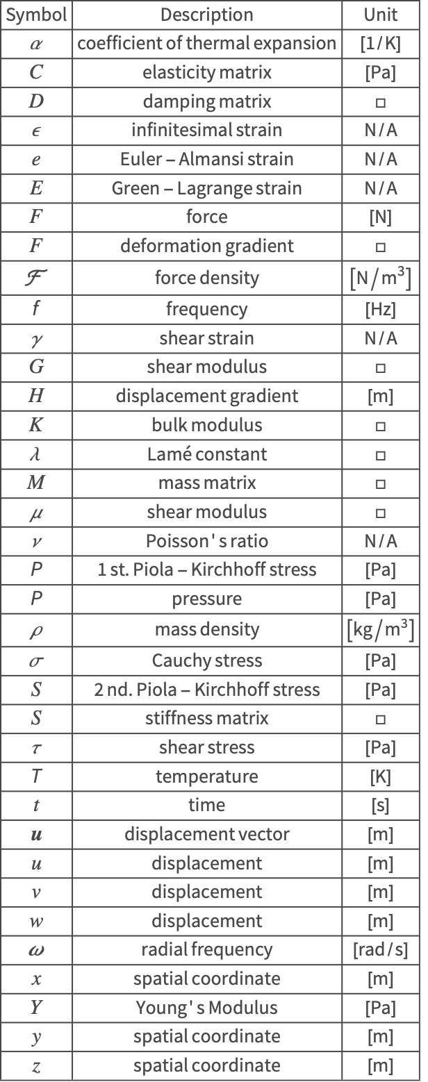
References
1. Backstrom, G; Simple Deformation and Vibration; GB Publishing; 2006
2. The Efficient Engineer, https://www.youtube.com/watch?v=aQf6Q8t1FQE; retrieved 2021/4/27
3. Cook, R et. al.; Concepts and Applications of Finite Element Analysis; Wiley 2002; 4th Edition
4. Bhatti, M.; Fundamental Finite Element Analysis and Application; Wiley 2005
5. Bhatti, M.; Advanced Topics in Finite Element Analysis of Structures; Wiley 2006
6. Brand, M.; Grundlagen FEM mit Solidworks; Vieweg+Teuber 2011; ISBN: 978-3-8348-1306-0
7. https://en.wikipedia.org/wiki/Modal_analysis_using_FEM, retrieved 01/06/2021
8. Nasdala, L.; FEM-Formelsammlung Statik und Dynamik; Vieweg+Teuber 2010
9. Alawadhi, E. M.; Finite Element Simulations Using ANSYS; CRC Press 2010
10. Constantinescu, A. and Korsunsky A.; Elasticity with Mathematica; Cambridge University Press 2007
11. Bower, A.; Applied Mechanics of Solids; CRC Press 2010; ISBN-13: 978-1439802472 http://solidmechanics.org/contents.php
12. The Efficient Engineer, https://www.youtube.com/watch?v=xkbQnBAOFEg; retrieved 2021/9/13
13. Kelly, P. A.; Mechanics Lecture Notes: An introduction to Solid Mechanics. http://homepages.engineering.auckland.ac.nz/~pkel015/SolidMechanicsBooks/index.html
14. Moosbrugger, C. (ed.); Atlas of Stress-Strain Curves; ASM International 2002; ISBN 0-87170-739-Xl https://books.google.com/books?id=up5KS9fd_pkC
15. Sifakis, E. and Barbič, J.; Finite Element Method Simulation of 3D Deformable Solids; M&C Publishers 2016; ISBN 9781627054423
16. Holzapfel, A.; Nonlinear Solid Mechanics; Wiley 2020; ISBN 978-0-471-82319-3
17. Bonet, J., Wood, R.; Nonlinear Continuum Mechanics for Finite Element Analysis; Cambridge University Press 1997; ISBN 0-521-57272-X
18. Mooney, M. "Large Elastic Deformations of Isotropic Materials." Journal of Applied Physics 1940. 11: 582–592. https://doi.org/10.1063/1.1712836
19. Rivlin, R. S. "Large Elastic Deformations of Isotropic Materials." Philosophical Transactions of the Royal Society of London. Mathematical and Physical Sciences 1948. 241: pp. 379–397. https://doi.org/10.1098/rsta.1948.0024
20. Arruda, M. Boyce, M. "A Three-Dimensional Constitutive Model for the Large Stretch Behavior of Rubber Elastic Materials." Journal of the Mechanics and Physics of Solids. 1993. Volume 41, Issue 2. pp. 389–412. https://doi.org/10.1016/0022-5096(93)90013-6
21. Gent, A. N. "A New Constitutive Relation for Rubber." Rubber Chemistry and Technology. 1996. 69 (1): 59–61. https://doi.org/10.5254/1.3538357
22. Treolar, L. R. G. "Stress-Strain Data for Vulcanised Rubber under Various Types of Deformation." Transactions of the Faraday Society, 1943
23. Ning, X., Zhu, Q., Lanir, Y. and Margulies, S. S. "A Transversely Isotropic Viscoelastic Constitutive Equation for Brainstem Undergoing Finite Deformation." Journal of Biomechanical Engineering, 2006. 128: pp. 925–933. DOI: 10.1115/1.2354208
24. Spencer, A. J. M.; Deformations of Fibre-Reinforced Materials; 1972
25. Nekliudova, E. A., Semenov, A. S., Melnikov, B. E. and Semenov, S. G. "Experimental Research and Finite Element Analysis of Elastic and Strength Properties of Fiberglass Composite Material." Magazine of Civil Engineering 3 (47), 2014
26. Otero, F., Oller, S., Martinez, X. and Salomón, O. "Numerical Homogenization for Composite Materials Analysis. Comparison with other Micro Mechanical Formulations." Composite Structures. 2015 Apr 1;122:405-16.
27. Charalambakis, N. "Homogenization Techniques and Micromechanics: A Survey and Perspectives." 2010: 030803.
28. Pascon, J. P. (2019). "Large Deformation Analysis of Plane-Stress Hyperelastic Problems via Triangular Membrane Finite Elements." International Journal of Advanced Structural Engineering, vol 3, pp. 331–350, https://doi.org/10.1007/s40091-019-00234-w.
29. Yosibash, Z., Weiss, D., and Hartmann, S. (2014). "High-Order FEMs for Thermo-hyperelasticity at Finite Strains." Computers and Mathematics with Applications, vol 67, pp. 477–496, https://doi.org/10.1016/j.camwa.2013.11.003
30. Wriggers, P.; Nonlinear Finite Element Methods; Springer 2008
31. Gasser, T. C.; Vascular Biomechanics: Concepts, Models and Applications; Springer 2021 https://doi.org/10.1007/978-3-030-70966-2
32. Ting, T. C.; Anisotropic Elasticity: Theory and Applications. Vol. 45. Oxford University Press, 1996