Hyperelasticity
Contents
Introduction
Materials like rubber or foam can be exposed to large deformations and still remain fully elastic. This means that if the load is removed, the deformation is fully reversible with no plastic deformation. These materials are called hyperelastic materials or Green elastic materials. Beyond rubber and foam, some biological tissue or polymers, which can have rubbery regimes, can also fall into the hyperelastic material category. In contrast to hypoelastic materials, hyperelastic materials can be subjected to large deformations and rotations.
For small deformations, the difference in shape between the object before and after the deformation is small compared to the size of the object. In the case of large deformations, that is no longer the case, and the deformation needs to be accounted for. For example, a large deformation may have an effect on the shape of a surface a force is acting on or the volume of the entire object. In the case of small deformations, this shape or volume change is neglected because it is negligible.
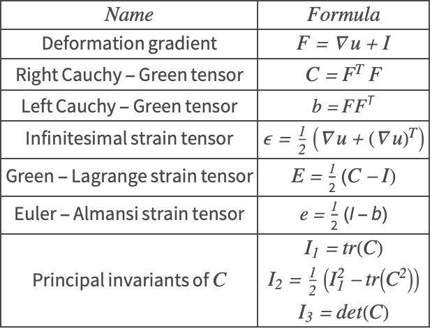
The mathematics behind large deformations is introduced in the section Deformation Gradient. Before proceeding, here is a summary of terms relevant in this section and their formulas:
Up until now, the only stress measure encountered was the Cauchy stress ![]() . Cauchy stress is a stress measure defined in the deformed configuration of an object under load. This deformed configuration is also called the spatial configuration. Ultimately, concerning the computation of a stress in an object, the computation of the Cauchy stress is the desired result. For hyperelastic material models, however, other stress measures are also used. This is because typically, it is much harder to define the model setup in the deformed configuration; it is preferable to define the model setup in the undeformed configuration. This undeformed configuration is also called the material or reference configuration. Once the stress in the undeformed configuration has been computed, it is possible to obtain the Cauchy stress and the procedure for doing this will be shown later. For now, it is important to know that the equilibrium equation relates a force density
. Cauchy stress is a stress measure defined in the deformed configuration of an object under load. This deformed configuration is also called the spatial configuration. Ultimately, concerning the computation of a stress in an object, the computation of the Cauchy stress is the desired result. For hyperelastic material models, however, other stress measures are also used. This is because typically, it is much harder to define the model setup in the deformed configuration; it is preferable to define the model setup in the undeformed configuration. This undeformed configuration is also called the material or reference configuration. Once the stress in the undeformed configuration has been computed, it is possible to obtain the Cauchy stress and the procedure for doing this will be shown later. For now, it is important to know that the equilibrium equation relates a force density ![]()
![]() to the first Piola–Kirchhoff stress
to the first Piola–Kirchhoff stress ![]()
![]() . The equation of motion in the reference configuration is given as:
. The equation of motion in the reference configuration is given as:
Here ![]() and
and ![]() , are the body force density and the mass density, both in the undeformed configuration. The term density in this context describes a quantity divided by the initial volume of material
, are the body force density and the mass density, both in the undeformed configuration. The term density in this context describes a quantity divided by the initial volume of material ![]() .
. ![]() is the unknown displacement vector.
is the unknown displacement vector. ![]() is the first Piola–Kirchhoff stress measured in [
is the first Piola–Kirchhoff stress measured in [![]() ] and is also defined in the undeformed configuration, so it is a force per undeformed area
] and is also defined in the undeformed configuration, so it is a force per undeformed area ![]() . The first Piola–Kirchhoff stress is often abbreviated with PK1.
. The first Piola–Kirchhoff stress is often abbreviated with PK1.
So far, the first Piola–Kirchhoff stress has been used for the equilibrium equation to express the setup in the initial configuration. The Cauchy stress is the current force per current area ![]() and is available in the deformed, final configuration. Unfortunately, there is more to it than that.
and is available in the deformed, final configuration. Unfortunately, there is more to it than that.
The general procedure for establishing a hyperelastic material model is to start from a scalar strain energy density function ![]() . The strain energy density function
. The strain energy density function ![]() is constructed from experiments and defines a given material. It is a measure of the energy stored in the material due to a deformation. This energy density function per unit undeformed volume is formulated as a function of a strain measure. The energy density function is then differentiated with respect to that strain measure and results in a stress measure.
is constructed from experiments and defines a given material. It is a measure of the energy stored in the material due to a deformation. This energy density function per unit undeformed volume is formulated as a function of a strain measure. The energy density function is then differentiated with respect to that strain measure and results in a stress measure.
Materials are considered elastic if their constitutive behavior can be expressed as a function of the current state of deformation only. When this condition holds, the stress measure of a particle at position ![]() is a function of the current deformation gradient
is a function of the current deformation gradient ![]() . The deformation gradient
. The deformation gradient ![]() is conjugate to the first Piola–Kirchhoff stress
is conjugate to the first Piola–Kirchhoff stress ![]() and it can be written:
and it can be written:
The double contraction ![]() of a stress tensor
of a stress tensor ![]() with the associated rate of deformation tensor
with the associated rate of deformation tensor ![]() describes the rate of internal mechanical work per unit reference volume. A strain energy density function is then given by [17, c. 5.2, p. 142]:
describes the rate of internal mechanical work per unit reference volume. A strain energy density function is then given by [17, c. 5.2, p. 142]:
Constitutive equations must describe relationships between compatible stress and strain measures [5, p. 498]. The first Piola–Kirchhoff stress ![]() and the deformation gradient
and the deformation gradient ![]() are such a compatible stress-strain pair. A strain energy density function can be expressed in equivalent forms in terms of different strain measures.
are such a compatible stress-strain pair. A strain energy density function can be expressed in equivalent forms in terms of different strain measures.
Constitutive behavior of solids is often given in terms of the material coordinates; the Lagrangian description is often preferred in solid mechanics [16, p. 61]. Since in solid mechanics setups, some aspects of the current configuration are generally not easily known, it is not convenient to work with stress tensors expressed in terms of the spatial configuration. In most cases, it is easier to work with stress tensors that are expressed in the reference configuration or an intermediate configuration [16, p. 109, p. 146]. To express the energy density function not only with the PK1 and the deformation gradient ![]() but also with the right Cauchy–Green deformation tensor
but also with the right Cauchy–Green deformation tensor ![]() , a new pseudo stress measure
, a new pseudo stress measure ![]() is introduced.
is introduced. ![]() is the second Piola–Kirchhoff stress measured in [
is the second Piola–Kirchhoff stress measured in [![]() ]. The second Piola–Kirchhoff stress is often abbreviated with PK2. The term pseudo stress means that this stress is defined neither in the undeformed nor in the deformed configuration.
]. The second Piola–Kirchhoff stress is often abbreviated with PK2. The term pseudo stress means that this stress is defined neither in the undeformed nor in the deformed configuration.
Like the stress field ![]() is said to be work conjugate to the strain field
is said to be work conjugate to the strain field ![]() , the stress field
, the stress field ![]() is said to be work conjugate to the strain field
is said to be work conjugate to the strain field ![]() [16, p. 155ff]. In other words, the Green–Lagrange strain
[16, p. 155ff]. In other words, the Green–Lagrange strain ![]() is compatible with the second Piola–Kirchhoff stress
is compatible with the second Piola–Kirchhoff stress ![]() [17, c. 5.2, p. 143]:
[17, c. 5.2, p. 143]:
Several other stress and work conjugates strains exist but will not be explored here.
As explained above, a strain energy density function can be expressed in equivalent forms in terms of different strain measures. For example, the energy density function ![]() is expressed in term of the Green–Lagrange strain
is expressed in term of the Green–Lagrange strain ![]() . Other possibilities for expressing an energy density function are to use, for example, the Cauchy tensors
. Other possibilities for expressing an energy density function are to use, for example, the Cauchy tensors ![]() , the infinitesimal strain
, the infinitesimal strain ![]() or invariants of
or invariants of ![]() . Depending on how the energy density function is expressed, for example,
. Depending on how the energy density function is expressed, for example, ![]() , the energy function is then differentiated with respect to that independent variable, for example,
, the energy function is then differentiated with respect to that independent variable, for example, ![]() .
.
If the strain energy density function is expressed in terms of the deformation gradient ![]() and the derivative of the strain energy density function is taken with respect to the deformation gradient
and the derivative of the strain energy density function is taken with respect to the deformation gradient ![]() , it leads to the PK1 stress:
, it leads to the PK1 stress:
since the deformation gradient ![]() is compatible with the first Piola–Kirchhoff stress
is compatible with the first Piola–Kirchhoff stress ![]() .
.
Differentiating a strain energy density ![]() that is a function of the Green–Lagrange strain
that is a function of the Green–Lagrange strain ![]() , the Cauchy deformation tensor
, the Cauchy deformation tensor ![]() or the infinitesimal strain
or the infinitesimal strain ![]() with respect to the strain measure will result in a second Piola–Kirchhoff stress
with respect to the strain measure will result in a second Piola–Kirchhoff stress ![]()
since the strain measures ![]() ,
, ![]() and
and ![]() are compatible with the second Piola–Kirchhoff stress
are compatible with the second Piola–Kirchhoff stress ![]() .
.
If the energy density function is expressed in a form that is compatible with a second Piola–Kirchhoff stress ![]() , it needs to be converted to a first Piola–Kirchhoff stress
, it needs to be converted to a first Piola–Kirchhoff stress ![]() such that it can be used in the equilibrium equation:
such that it can be used in the equilibrium equation:
A resulting second Piola–Kirchhoff stress ![]() can be converted to a first Piola–kirchhoff stress
can be converted to a first Piola–kirchhoff stress ![]() with the relation:
with the relation:
The equilibrium equation is then:
Nanson's formulas describe how stresses can be converted into each other and are summarized in the following list [5, p. 482]:
What complicates matters further with regard to reading literature is that some authors define the stress differently, in that they use a transposed version [11, ch2.2.3 p. 44]. It is possible to use, for example, ![]() , where the second subscript
, where the second subscript ![]() corresponds to the surface normal vector.
corresponds to the surface normal vector.
The transformation of quantities between the material and spatial configurations are called push-forward and pull-back operations [16, p. 82].
- The first Piola–Kirchhoff stress is used for the equilibrium equation, because entities need to be expressed in the initial configuration.
- The second Piola–Kirchhoff stress is commonly used for the constitutive equation, because the PK2 is compatible with the Green–Lagrange strain
 and the right Cauchy tensor
  .
.
As a side note, in the case of an infinitesimal strain measure ![]() , the stress measures
, the stress measures ![]() ,
, ![]() and
and ![]() are roughly the same, such that
are roughly the same, such that ![]() , and in that sense, the infinitesimal strain
, and in that sense, the infinitesimal strain ![]() is also compatible with the PK2
is also compatible with the PK2 ![]() . For this reason there is no need to differentiate these stresses in the linear elastic theory.
. For this reason there is no need to differentiate these stresses in the linear elastic theory.
Needs["NDSolve`FEM`"]
$HistoryLength = 0;vars = {{u[x, y, z], v[x, y, z], w[x, y, z]}, {x, y, z}};cubeMesh = ToElementMesh[Cuboid[], MaxCellMeasure -> 0.01, "MeshElementType" -> TetrahedronElement]St. Venant–Kirchhoff Model
The St. Venant–Kirchhoff model is a simple model of a hyperelastic material. The St. Venant–Kirchhoff model is a phenomenological model. This means it describes observed behavior. Its purpose is mainly educational, as it has deficiencies in the large deformation regime. In that case, the St. Venant–Kirchhoff model softens under compression that is not physical. Here, the St. Venant–Kirchhoff model is used as an example to introduce formulating custom constitutive equations.
The simplest constitutive model is linear elasticity. Defined in terms of the strain, energy density is given as [14, p 13]:
where ![]() is the infinitesimal strain tensor,
is the infinitesimal strain tensor, ![]() is the first Lamé constant and
is the first Lamé constant and ![]() is the second constant, also known as shear modulus
is the second constant, also known as shear modulus ![]() . The Lamé constants can be related to the Young modulus and Poisson ratio, as shown in the section on Alternative Material Parameters.
. The Lamé constants can be related to the Young modulus and Poisson ratio, as shown in the section on Alternative Material Parameters. ![]() is the corresponding energy density function for linear elasticity.
is the corresponding energy density function for linear elasticity.
The St.Venant–Kichhoff model uses the above energy density function but uses the Green–Lagrange strain ![]() in place of the infinitesimal strain tensor
in place of the infinitesimal strain tensor ![]() .
.
For the Green–Lagrange strain ![]() , the energy density function
, the energy density function ![]() is given as [14, p 15]:
is given as [14, p 15]:
The derivative of the energy density function ![]() with respect to the Green–Lagrange strain
with respect to the Green–Lagrange strain ![]() is:
is:
where ![]() is the second Piola–Kirchhoff stress and
is the second Piola–Kirchhoff stress and ![]() is the identity matrix.
is the identity matrix.
ESymbol = MatrixSymbol["E", {3, 3}];
D[1 / 2 * λ * Tr[ESymbol] ^ 2 + μ * Tr[ESymbol.ESymbol], ESymbol]
Hyperelastic material laws are highly nonlinear, which can make them very challenging to solve. Depending on the amount of the final deformation, it is unrealistic to expect any solver to find a solution with the standard approach of iteratively solving a set of linearized equations. This is not a problem of the Wolfram Language specifically, but a challenge any PDE solving functionality faces. To work with this challenge, two main workflows are available. In both approaches, the force acting on the object is slowly increased. The two approaches are
The first approach is to create a parametric function with a parameter ![]() that has an influence on the amount of deformation. Initially, this parameter
that has an influence on the amount of deformation. Initially, this parameter ![]() may be set to 0, and a solution to the system of equations is obtained. This solution is then used as an initial seed for the next evaluation of the parametric system, where
may be set to 0, and a solution to the system of equations is obtained. This solution is then used as an initial seed for the next evaluation of the parametric system, where ![]() is slightly increased. That solution is then reused in the same manner until the parameter
is slightly increased. That solution is then reused in the same manner until the parameter ![]() reaches 1, which is equivalent to the full displacement of the system. This procedure was already made use of in the section about Hypoelastic Models.
reaches 1, which is equivalent to the full displacement of the system. This procedure was already made use of in the section about Hypoelastic Models.
The second approach uses time integration to achieve the same thing: slowly increase the amount of force acting on the object. The main advantage of using time integration is that NDSolve has an adaptive time step mechanism that choses the next time step automatically. In the parametric force increment approach, one has to choose the size of a next step manually, which is not the case for the pseudo time integration method. Here the system of equations is integrated from 0 to 1, which is an arbitrarily chosen end time. Time variable ![]() now takes the place of the parameter
now takes the place of the parameter ![]() and is used to slowly increase the force acting on the object. This approach will be shown in the section discussing the neo-Hookean material model. The following examples shows the parametric force increment approach.
and is used to slowly increase the force acting on the object. This approach will be shown in the section discussing the neo-Hookean material model. The following examples shows the parametric force increment approach.
As an example, a unit cube is used. The cube is under tension in the positive ![]() direction while at the same time fixed at
direction while at the same time fixed at ![]() .
.
parsStVKI = <|"SolidMechanicsMaterialModel" -> "VenantKirchhoff", "LameParameter" -> 100, "ShearModulus" -> 1|>;pfunStVKI = ParametricNDSolveValue[{SolidMechanicsPDEComponent[vars, parsStVKI] == {0, 0, 0}
, SolidFixedCondition[x == 0, vars, parsStVKI]
, SolidDisplacementCondition[x == 1, vars, parsStVKI, <|"Displacement" -> {p, None, None}|>]}, vars[[1]], {x, y, z}∈cubeMesh, p]pMax = 0.2;
nsteps = 40;
displacementStVKI = {0, 0, 0};In the following, the previous solution is used to start the nonlinear solve for the current solution.
Monitor[Do[
	pNew = step * pMax / nsteps;
	displacementStVKI = pfunStVKI[pNew, "InitialSeeding" -> Thread[Equal[vars[[1]], displacementStVKI]]];
	, {step, 1, nsteps, 1}],
	step];
Should the nonlinear solver not converge, the first thing to try is to increase nsteps, the number of steps taken. That the solver does not converge can have many causes. Even increasing the number of elements can make a solver fail to find a solution that it did find with fewer elements. In that case, one option is to use a coarse mesh, find a solution and use that as an initial seed for a fine grid computation. This approach is shown in the finite element best practice Solving Memory-Intensive PDEs. The example there uses an iterative solver, but the default linear solve can be used by removing the option that specifies the iterative solver.
For hyperelastic material models, one often wants to see the deformation to scale, since the deformations are large and visible. For this, the "ScalingFactor" of the deformation or the original geometry can be set to 1.
deformedMeshStVKI = ElementMeshDeformation[cubeMesh, displacementStVKI, "ScalingFactor" -> 1];The following visualization is to scale.
Show[cubeMesh["Edgeframe"], deformedMeshStVKI["Wireframe"["ElementMeshDirective" -> Directive[Opacity[0.2], Red]]]]NIntegrate[1, {x, y, z}∈deformedMeshStVKI]The volume is smaller than the initial volume. More on this topic can be found in the section on Compressibility.
strainsStVKI = SolidMechanicsStrain[vars, parsStVKI, displacementStVKI];Computing the Cauchy stress from the strain works a little bit differently than in the linear elastic case. In the linear elastic case, it is possible to use the strain to recover the stress. Now, since the constitutive equations work with the second Piola–Kirchhoff stress, the deformation gradient ![]() is also needed to convert it to a Cauchy stress.
is also needed to convert it to a Cauchy stress.
cauchyStressStVKI = SolidMechanicsStress[vars, parsStVKI, strainsStVKI, displacementStVKI];If the stress you are interested in is the same as the stress the constitutive equation uses, which is the case for linear elastic material, then and only then, no displacement needs to be given.
SolidMechanicsStress[vars, Join[parsStVKI, <|"OutputStressMeasure" -> "SecondPiolaKirchhoff"|>], strainsStVKI]SolidMechanicsStress[vars, Join[parsStVKI, <|"OutputStressMeasure" -> "FirstPiolaKirchhoff"|>], strainsStVKI, displacementStVKI]Note that the first Piola–Kirchhoff stress is not symmetric and cannot be used, for example, in visualizing a von Mises stress, since that requires that the tensor used be symmetric.
vonMisesStress = VonMisesStress[vars, parsStVKI, cauchyStressStVKI]vonMisesStressFunction = Head[vonMisesStress]MinMax[vonMisesStressFunction["ValuesOnGrid"]]Visualizing the von Mises stress over the deformed object is desired.
deformedVonMisesStressStVKI = ElementMeshInterpolation[deformedMeshStVKI, vonMisesStressFunction["ValuesOnGrid"]];Show[cubeMesh["Edgeframe"],
deformedMeshStVKI["Edgeframe"],
SliceContourPlot3D[deformedVonMisesStressStVKI[x, y, z], deformedMeshStVKI, {x, y, z}∈deformedMeshStVKI, ...]]Next, the objective is to see if linear elasticity can be reproduced using the St. Venant–Kirchhoff model. For the infinitesimal strain ![]() , the energy density function
, the energy density function ![]() is given as [14, p 13]:
is given as [14, p 13]:
![]() is the first Lamé constant and
is the first Lamé constant and ![]() is the second constant, also known as shear modulus
is the second constant, also known as shear modulus ![]() . The Lamé constants can be related to the Young modulus and Poisson ratio.
. The Lamé constants can be related to the Young modulus and Poisson ratio.
The derivative of the energy density function ![]() with respect to the infinitesimal strain
with respect to the infinitesimal strain ![]() is:
is:
pdeModel[vars_, pars_] := {SolidMechanicsPDEComponent[vars, pars] == {0, 0, 0},
	SolidFixedCondition[x == 0, vars, pars],
	SolidDisplacementCondition[x == 1, vars, pars, <|"Displacement" -> {0.01, None, None}|>]
}basePars = <|"YoungModulus" -> 10 ^ 8, "PoissonRatio" -> 0.3|>;parsStVKI = Join[<|"SolidMechanicsMaterialModel" -> "VenantKirchhoff", "StrainMeasure" -> "Infinitesimal"|>, basePars];displacementStVKI = NDSolveValue[pdeModel[vars, parsStVKI], {u, v, w}, {x, y, z}∈cubeMesh];Next, the same model setup is computed using the linear elastic functionality. To make stresses better comparable, the typical engineering strain used for linear elastic materials is not used. It is possible to switch off the usage of engineering strains by setting "EngineeringStrain"False in the parameters pars. This may be of interest when comparing linear material laws with nonlinear material laws, where true stain is used. More information can be found in the reference page of SolidMechanicsStrain.
parsLinear = Join[<|"EngineeringStrain" -> False|>, basePars];displacementLinear = NDSolveValue[pdeModel[vars, parsLinear], {u, v, w}, {x, y, z}∈cubeMesh];minmax[displacement_] := MinMax /@ Through[displacement["ValuesOnGrid"]]
minmax[displacementStVKI] - minmax[displacementLinear]The St. Venant–Kirchhoff model has limits. The model has poor resistance to forceful compression. As a St. Venant–Kirchhoff elastic body is compressed, it initially reacts with a restorative force. Beyond a critical compression threshold (≈58% of undeformed dimensions along a single axis), the restorative force decreases [15]. In other words, the St. Venant–Kirchhoff model becomes softer when it is compressed.
To give more information on how to write user-defined material laws, it can be instructive to see actual implementations. An example of how to add a user-defined material law, sometimes called UMAT, was shown in the section on hypoelastic materials. The actual implementation of the St. Venant–Kirchhoff material model is given below, and the way this model is constructed can be used as an example for constructing other constitutive models.
MaterialModel[_, "Isotropic", "VenantKirchhoff", vars_, pars_, data__] :=

Module[
    {X, dim, lambda, mu, EE, ee, rules, stressMatrix, strainMeasure},

    values = GetSolidMechanicsMaterialParameterList[vars, pars,
        {"LameParameter", "ShearModulus"}, <||>];
    If[ FailureQ[values], Return[ $Failed, Module]; ];
    {lambda, mu} = values;

    X = vars[[-1]];
    dim = Length[X];
    EE = Array[ee, {dim, dim}];
    stressMatrix = lambda * Tr[EE] * IdentityMatrix[dim] + 2 * mu * EE;

    (* get the strain measure *)
    strainMeasure = "StrainMeasure" /. data;
    rules = Thread[Rule[Flatten[EE], Flatten[strainMeasure]]];
    stressMatrix = stressMatrix /. rules;

    stressMatrix
]
Adding a New Material Model
Now that a first hyperelastic material model has been examined, the process of creating a new material model can be demonstrated. The previously introduced St. Venant–Kirchhoff model will be used to illustrate how to incorporate it as a custom model.
MyMaterialModel[varsIn_, parsIn_, data__]  :=
Module[
	{X, dim, lambda, mu, EE, ee, rules, stressMatrix, strainMeasure},
	Print["Hello World"];

	lambda = PDEModels`GetSolidMechanicsMaterialParameter[varsIn, parsIn, "LameParameter"];
	If[FailureQ[lambda], Return[$Failed, Module];];

	mu = PDEModels`GetSolidMechanicsMaterialParameter[varsIn, parsIn, "ShearModulus"];
	If[FailureQ[mu], Return[$Failed, Module];];

	X = varsIn[[-1]];
	dim = Length[X];
	EE = Array[ee, {dim, dim}];
	stressMatrix = (lambda * Tr[EE] * IdentityMatrix[dim]) + 2 * mu * EE;
	strainMeasure = "StrainMeasure" /. data;
	rules = Thread[Flatten[EE] -> Flatten[strainMeasure]];
	stressMatrix = stressMatrix /. rules;
	stressMatrix
	]
Once a material model is established, the solid mechanics functions need to be instructed on how to utilize it. This is achieved by specifying the proper parameters in the parameter association.
parsMyModel = <|"SolidMechanicsMaterialModelFunction" -> MyMaterialModel,
	"LameParameter" -> 100, "ShearModulus" -> 1,
	"StrainMeasure" -> "GreenLagrange",
	"ConstitutiveStressMeasure" -> "SecondPiolaKirchhoff",
	"EquilibriumStressMeasure" -> "FirstPiolaKirchhoff"|>;
The "SolidMechanicsMaterialModelFunction" specifies the new material model. The material parameters are the same as above for the St. Venant–Kirchhoff example. As a "StrainMeasure", the "GreenLagrange" strain is used. More information on the available strain measures can be found in the theory section on strain. Next, the stress measure used in the material law needs to be specified for SolidMechanicsPDEComponent. "ConstitutiveStressMeasure" is the stress measure used for the material law. "EquilibriumStressMeasure" is the stress measure of the nonlinear equilibrium equation. For example, to specify the material law with "FirstPiolaKirchhoff" stress, the "ConstitutiveStressMeasure" would then be set accordingly. The "OutputStressMeasure" is, by default, the "Cauchy" stress but can be changed. The conversions between the stresses happen automatically.
Neo-Hookean Model
As the name suggests, the neo-Hookean material model is an extension of the linear elastic Hooke model to large deformations. The energy density function for a compressible neo-Hookean model ![]() is given as [5, p. 499]:
is given as [5, p. 499]:
Various other formulations for the same energy density function exist and are usually based on invariants, for example
where ![]() is the first invariant and
is the first invariant and ![]() , but will not be pursued here. The second Piola–Kirchhoff stress is given as [5, p. 500]:
, but will not be pursued here. The second Piola–Kirchhoff stress is given as [5, p. 500]:
To give more information on how to write user-defined material laws, it can be instructive to see actual implementations. An example of how to add a user-defined material law, sometimes called UMAT, was shown in the section on hypoelastic materials. The actual implementation of the neo-Hookean material law is given in a more detailed section on the neo-Hookean model. The way this model is constructed can be used as an example for constructing other constitutive models.
The neo-Hookean model is a mechanistic model. This means it is derived from the mechanical principles of the material. Sometimes, the coefficients ![]() , where
, where ![]() is the shear modulus, and
is the shear modulus, and ![]() , with
, with ![]() the bulk modulus, are made use of.
the bulk modulus, are made use of.
As an example, a unit cube is used. The cube is under tension in the positive ![]() direction while at the same time fixed at
direction while at the same time fixed at ![]() . The body is stretched by 40%.
. The body is stretched by 40%.
pdeModel[vars_, pars_] := {SolidMechanicsPDEComponent[vars, pars] == {0, 0, 0},
	SolidFixedCondition[x == 0, vars, pars],
	SolidDisplacementCondition[x == 1, vars, pars, <|"Displacement" -> {p, None, None}|>]
	}
The model under discussion here is a compressible model. This means that the volume of the deformed object may change when under load. A compressible model is in contrast to an incompressible or a nearly incompressible model, which will be discussed later. The default for the implemented hyperelastic material models is to be nearly incompressible. To make use of the model discussed here, the parameter "Compressibility"->"Compressible" has to be specified.
C10 = 2881;D1 = 10 ^ -6;
parsNeoHook = <|"SolidMechanicsMaterialModel" -> "NeoHookean", "ShearModulus" -> 2 * C10, "BulkModulus" -> 2 / D1, "MassDensity" -> 980, "Compressibility" -> "Compressible"|>;
First, try the parametric force increment approach.
pfunNeoHook = ParametricNDSolveValue[pdeModel[vars, parsNeoHook], {u, v, w}, {x, y, z}∈cubeMesh, p];pfunNeoHook[0.4 / 100]Even a small initial increment in the boundary displacement fails to converge. While it is possible to decrease the initial displacement further to get to a converging solution, iterating that solution forward to the 40% stretch is going to take a long time if the step size remains small. As an alternative, the PDE is converted to a time-dependent PDE with an initial condition and a derivative of the initial condition of 0 to time-integrate the PDE model to a fictitious time of 1 unit.
tEnd = 1;
tvars = {{u[t, x, y, z], v[t, x, y, z], w[t, x, y, z]}, t, {x, y, z}};
AbsoluteTiming[Monitor[transientDisplacementNeoHook = NDSolveValue[{pdeModel[tvars, parsNeoHook] /. p -> 0.4 * t, #[0, x, y, z] == 0& /@ {u, v, w}, Derivative[1, 0, 0, 0][#][0, x, y, z] == 0& /@ {u, v, w}},
	{u, v, w}, {t, tEnd, tEnd}, {x, y, z}∈cubeMesh, EvaluationMonitor :> (monitor = Row[{"t = ", CForm[t]}])],
	monitor
	];]
Typically, when specifying the time range for a time-dependent differential equation in NDSolve or its related functions, it is specified as a list of time variable ![]() , the start time and the end time,
, the start time and the end time, ![]() . In the above call to NDSolveValue, the time domain is specified as
. In the above call to NDSolveValue, the time domain is specified as ![]() . Note that
. Note that ![]() is set to
is set to ![]() . This means that the time integration is still performed from the time the initial conditions give to the final time
. This means that the time integration is still performed from the time the initial conditions give to the final time ![]() , but at the same time, this instructs NDSolveValue to just store the last time step
, but at the same time, this instructs NDSolveValue to just store the last time step ![]() in the resulting interpolating function.
in the resulting interpolating function.
In order to make the subsequent processing of the data more efficient, the time-dependent interpolating functions of the displacement are converted to stationary interpolating functions. This is easy to do in this case, since only the last time step is of interest. InterpolatingFunction objects store the solution of all nodes at the various time steps NDSolve has taken in a list. Only the last set of values is extracted from the interpolating function. These values can then be packaged into new interpolating functions.
displacementNeoHook = ElementMeshInterpolation[cubeMesh, Last[#["ValuesOnGrid"]]]& /@ transientDisplacementNeoHook;deformedMeshNeoHook = ElementMeshDeformation[cubeMesh, displacementNeoHook, "ScalingFactor" -> 1]NIntegrate[1, {x, y, z}∈deformedMeshNeoHook]The volume is larger then the initial volume. More on this topic can be found in the section on Compressibility. The volume increase is, however, small compared to the overall volume.
Show[cubeMesh["Edgeframe"], deformedMeshNeoHook["Wireframe"["ElementMeshDirective" -> Directive[Opacity[0.2], Red]]]]deformedDisplacementNeoHook = ElementMeshInterpolation[deformedMeshNeoHook, #["ValuesOnGrid"]][x, y, z]& /@ displacementNeoHook;SliceContourPlot3D[Sqrt[Total[deformedDisplacementNeoHook ^ 2]]//Evaluate, deformedMeshNeoHook, {x, y, z}∈deformedMeshNeoHook, ColorFunction -> "Temperature", PlotLegends -> Automatic]Note that in the above graphic the bounding box of the graphic is shown and not the original undeformed cube.
strainsNeoHook = SolidMechanicsStrain[vars, parsNeoHook, displacementNeoHook]AbsoluteTiming[cauchyStressNeoHook = SolidMechanicsStress[vars, parsNeoHook, strainsNeoHook, displacementNeoHook]]vonMisesStress = VonMisesStress[vars, parsNeoHook, cauchyStressNeoHook]vonMisesStressFunction = Head[vonMisesStress]MinMax[vonMisesStressFunction["ValuesOnGrid"]]deformedVonMisesStressNeoHook = ElementMeshInterpolation[deformedMeshNeoHook, vonMisesStressFunction["ValuesOnGrid"]];Show[cubeMesh["Edgeframe"],
deformedMeshNeoHook["Edgeframe"],
SliceContourPlot3D[deformedVonMisesStressNeoHook[x, y, z], deformedMeshNeoHook, {x, y, z}∈deformedMeshNeoHook, ...], ViewPoint -> {-2, -2, 1}]The contours are numerical artefacts resulting from the coarse mesh used.
The neo-Hookean model is also used in the Biaxial Tensile Test Hyperelastic Tissue application model.
MaterialModel[_, "Isotropic", "NeoHookeanCompressible", vars_, pars_, data__]:=
Module[
    {U, X, dim, lambda, mu, fp, f, idm, c, cinv, j, stressMatrix},

    values = GetSolidMechanicsMaterialParameterList[vars, pars,
        {"LameParameter", "ShearModulus"}, <||>];
    If[ FailureQ[values], Return[ $Failed, Module]; ];
    {lambda, mu} = values;

    dim = pars["EmbeddingDimension"];
    idm = IdentityMatrix[3];
    f = idm;
    f[[1 ;; dim, 1 ;; dim]] = DeformationGradient[vars, pars];

    (* in the plane strain case: f[[3,3]] = 1; *)
    If[ pars["SolidMechanicsModelForm"] == "PlaneStress",
        f[[3,3]] = Exp[-lambda/(lambda + 2 mu) Log[Det[f[[1;;dim, 1;;dim]]]]];
    ];

    j = Det[f];
    c = Transpose[f] . f;
    cinv = Inverse[c];
    stressMatrix = mu * (idm - cinv) + lambda * Log[j] * cinv;

    (* Second Piola-Kirchhoff stress *)
    Simplify[stressMatrix[[1;;dim, 1;;dim]]]
]
Strain and Stress Invariants
The strain energy density function ![]() is often expressed through the Cauchy–Green strain
is often expressed through the Cauchy–Green strain ![]() instead of the deformation gradient
instead of the deformation gradient ![]() . In principal, using the deformation gradient
. In principal, using the deformation gradient ![]() is perfectly fine. The disadvantage, however, is that using
is perfectly fine. The disadvantage, however, is that using ![]() can be unintuitive when designing material models. For example, the compressibility of material models can be expressed well when using a different formulation than the deformation gradient
can be unintuitive when designing material models. For example, the compressibility of material models can be expressed well when using a different formulation than the deformation gradient ![]() to express the energy density function
to express the energy density function ![]() . It is thus common to express
. It is thus common to express ![]() through a strain measure, like the Cauchy–Green strain
through a strain measure, like the Cauchy–Green strain ![]() or though invariants that are derived from the deformation gradient
or though invariants that are derived from the deformation gradient ![]() [15, p. 11ff].
[15, p. 11ff].
The material models should be rotationally invariant. That means the model should give the same result if the object and loads are rotated. A hyperelastic material model is rotationally invariant if and only if the strain energy density function satisfies:
A second property is related to the isotropy of the materials. A material is called isotropic if its material properties are the same in all directions. A hyperelastic material model is isotropic if and only if the strain energy density function satisfies:
where ![]() is a rotation matrix. As a consequence, a material that is both rotationally invariant and isotropic satisfies:
is a rotation matrix. As a consequence, a material that is both rotationally invariant and isotropic satisfies:
Using a singular-value decomposition ![]() , a rotationally invariant and isotropic material satisfies:
, a rotationally invariant and isotropic material satisfies:
where ![]() is the three singular values of
is the three singular values of ![]() , namely
, namely ![]() ,
, ![]() and
and ![]() . The
. The ![]() are called the principal stretches. One could define the strain energy density function
are called the principal stretches. One could define the strain energy density function ![]() in terms of the singular values of
in terms of the singular values of ![]() , but this is not done for isotropic material since the computation of the singular-value decomposition is expensive. Instead, what is done is to use three isotropic invariants
, but this is not done for isotropic material since the computation of the singular-value decomposition is expensive. Instead, what is done is to use three isotropic invariants ![]() ,
, ![]() and
and ![]() of the Cauchy–Green strain tensor
of the Cauchy–Green strain tensor ![]() , which are as good as the singular values but easier to compute. The isotropic invariants are defined as
, which are as good as the singular values but easier to compute. The isotropic invariants are defined as
Here ![]() ,
, ![]() and
and ![]() are the first, second and third isotropic invariants, respectively, and
are the first, second and third isotropic invariants, respectively, and ![]() is the right Cauchy–Green deformation tensor. Note that in the literature, there are at least two ways to define
is the right Cauchy–Green deformation tensor. Note that in the literature, there are at least two ways to define ![]() :
:
The invariants can also be expressed making use of the principal stretches ![]() , which are the singular values of
, which are the singular values of ![]() :
:
A special case can be identified when there is no strain, all the stretches are ![]() and the invariants are constant
and the invariants are constant ![]() ,
, ![]() and
and ![]() , respectively.
, respectively.
In summary, the strain energy density function ![]() can be expressed both in terms of the Cauchy–Green strain and the strain invariants
can be expressed both in terms of the Cauchy–Green strain and the strain invariants ![]() :
:
The invariants return a unique measure of strain that does not depend on rotations and is cheap to compute.
In practice, it is also useful to know the derivatives of the invariants with respect to the right Cauchy–Green strain ![]() [16, p. 216]:
[16, p. 216]:
where ℐ represents the identity matrix.
From this, the second Piola–Kirchhoff stress ![]() can be derived from the invariants
can be derived from the invariants ![]() . For this, the strain energy density function
. For this, the strain energy density function ![]() is expressed though the isotropic invariants
is expressed though the isotropic invariants ![]() . The second Piola–Kirchhoff stress
. The second Piola–Kirchhoff stress ![]() can then be computed through the chain rule as:
can then be computed through the chain rule as:
Using the derivatives of the invariants the expression is simplified to:
Note that the concept of invariants extends beyond the strain tensor and can be applied to a general tensor. The notation remains the same and for a general tensor ![]() :
:
A special mention should be made of the invariants of the deviatoric part of a tensor. These often arise in the context of specific post-processing tasks or when defining material properties based on the stress state of the material. In this case, the invariants of the deviatoric tensor are commonly denoted by the letter ![]() .
.
Where the deviatoric operator is defined as:
If an invariant is introduced without explicitly stating its dependency, and no other specification is given in the subsequent text, it should be understood as referring to the Cauchy–Green strain tensor.
Compressibility
One important aspect of the description of materials is their volumetric behavior when they are deformed. Typically compressible, incompressible and nearly incompressible material models are separated. In a compressible material description, the volume of the deformed object is allowed to change. For an incompressible material, the change in volume under deformation is zero. This incompressibility is expressed by the mathematical definition of incompressibility and is given as ![]() .
.
An incompressible material model is, in a way, the equivalent of a linear elastic material with a Poisson ratio of ![]() , where the incompressibility is enforced by requiring that
, where the incompressibility is enforced by requiring that ![]() . A Poisson ratio
. A Poisson ratio ![]() expresses a material behavior in the direction perpendicular to the direction of loading. The Poisson ratio allows the relative change of volume due to the stretch as
expresses a material behavior in the direction perpendicular to the direction of loading. The Poisson ratio allows the relative change of volume due to the stretch as ![]() to be expressed. For incompressible materials, where the volume change is zero
to be expressed. For incompressible materials, where the volume change is zero ![]() , the Poisson ratio has to be
, the Poisson ratio has to be ![]() . This in turn leads to an infinite bulk modulus
. This in turn leads to an infinite bulk modulus ![]() and results in extra stiffness when solving the model. To avoid the numerical difficulty of solving the stiff models, nearly incompressible models have been introduced.
and results in extra stiffness when solving the model. To avoid the numerical difficulty of solving the stiff models, nearly incompressible models have been introduced.
To model incompressible materials, the strain energy density function ![]() is split into an isochoric, constant volume part
is split into an isochoric, constant volume part ![]() and a volumetric part
and a volumetric part ![]() :
:
where ![]() . The isochoric part
. The isochoric part ![]() represents deformations without changes in volume. The volumetric part
represents deformations without changes in volume. The volumetric part ![]() models the incompressibility. In fact, the volumetric part is used to enforce incompressibility.
models the incompressibility. In fact, the volumetric part is used to enforce incompressibility. ![]() is constructed such that it depends only on the volume ratio
is constructed such that it depends only on the volume ratio ![]() . A model that enforces
. A model that enforces ![]() is incompressible.
is incompressible.
![]() is given as
is given as ![]() [16, p. 230]. However, since
[16, p. 230]. However, since ![]() is imposed for incompressibility, this results in
is imposed for incompressibility, this results in ![]() .
. ![]() is used to indicate that the strain energy density function
is used to indicate that the strain energy density function ![]() depends only on isochoric deformations.
depends only on isochoric deformations.
For a fully incompressible material, the volumetric part ![]() is not defined but instead is postulated through a strain energy with a constraint. A hydrostatic pressure
is not defined but instead is postulated through a strain energy with a constraint. A hydrostatic pressure ![]() is introduced to enforce the incompressibility:
is introduced to enforce the incompressibility:
Differentiating ![]() with the chain rule
with the chain rule
gives ![]() and
and ![]() . Then with
. Then with ![]() , this leads to the second Piola–Kirchhoff stress
, this leads to the second Piola–Kirchhoff stress ![]() , which can now be expressed as:
, which can now be expressed as:
In the above differentiation, the isochoric part is differentiated with respect to ![]() , and the second term only depends on
, and the second term only depends on ![]() .
.
Enforcing ![]() exactly can be problematic numerically, since that increases the stiffness of the model. Additionally, it requires an extra degree of freedom. So, instead of aiming for an exact satisfaction
exactly can be problematic numerically, since that increases the stiffness of the model. Additionally, it requires an extra degree of freedom. So, instead of aiming for an exact satisfaction ![]() , the requirement is loosened and the aim is to achieve
, the requirement is loosened and the aim is to achieve ![]() . This is what is called a nearly incompressible model and is a good compromise. The volumetric part is now expressed as:
. This is what is called a nearly incompressible model and is a good compromise. The volumetric part is now expressed as:
to enforce the incompressibility constraint ![]() . The hydrostatic pressure
. The hydrostatic pressure ![]() can be expressed as:
can be expressed as:
where ![]() is the material's bulk modulus. If experimental values for
is the material's bulk modulus. If experimental values for ![]() are not available,
are not available, ![]() can be related to the shear modulus
can be related to the shear modulus ![]() by
by ![]() .
. ![]() is a scale factor and typically in the range
is a scale factor and typically in the range ![]() .
.
k = EstimateBulkModulus[vars, pars, <|s -> 10^4, "ShearModulus" -> mu|>];
p = - k * (j - 1);
The second Piola–Kirchhoff stress for a nearly incompressible material model is:
Hyperelastic Model Collection
The models presented here can be classified into phenomenological, mechanistic and hybrid models. A phenomenological description of a material means that the model is made in such a way that it matches experimental data as closely as possible but does not have a physical basis. In contrast, a mechanistic model is based on physical processes, and one tries to match experimental data. Hybrid models account for both aspects.
All the hyperelastic models presented below have model parameters. Some of them, like the shear modulus, are specified as string parameters like "ShearModulus". Other parameters that do not have names or are part of an equation are given as formal symbol parameters such as ![]() . The notational alphabet guide page explains how to create the formal symbols. As far as the workflow is concerned, the formal symbol variables can just be copied from the examples below.
. The notational alphabet guide page explains how to create the formal symbols. As far as the workflow is concerned, the formal symbol variables can just be copied from the examples below.
A comparison of the hyperelastic material models is available in the Hyperelastic Model Comparison application example.
Mooney–Rivlin Models
The generalized Rivlin hyperelastic model is commonly used to describe the mechanical behavior of rubberlike materials that exhibit significant nonlinear deformations. This model is suitable for materials that undergo large strains and possess isotropic, homogeneous and nearly incompressible properties. It is often employed in applications, including biomechanics, soft tissue mechanics and elastomer engineering and is considered a phenomenological model.
The strain energy density function ![]() of the generalized Rivlin [18] model is given as:
of the generalized Rivlin [18] model is given as:
with ![]() representing material coefficients related to the isochoric response of an applied stress. The coefficient
representing material coefficients related to the isochoric response of an applied stress. The coefficient ![]() is always set to 0, such that
is always set to 0, such that ![]() .
.
The last term in Eqn. (1) is related to the compressible version of the Mooney–Rivlin model, where ![]() is related to the volumetric response due to stress application. Since the current version of the Wolfram Language does not provide a compressible version,
is related to the volumetric response due to stress application. Since the current version of the Wolfram Language does not provide a compressible version, ![]() is set to
is set to ![]() .
.
To make the model consistent with linear elasticity, it is also necessary that the bulk modulus be set to ![]() and the shear modulus be set to
and the shear modulus be set to ![]() .
.
Special combinations of the indices ![]() and
and ![]() of the material coefficients
of the material coefficients ![]() lead to well-known models. For example, the two-parameters Mooney–Rivlin model with
lead to well-known models. For example, the two-parameters Mooney–Rivlin model with ![]() and
and ![]() ,
, ![]() ,
, ![]() or with
or with ![]() leads to the neo-Hookean model. The most commonly used versions are the two-, five- and nine-parameters versions of the Mooney–Rivlin.
leads to the neo-Hookean model. The most commonly used versions are the two-, five- and nine-parameters versions of the Mooney–Rivlin.
The incompressible Mooney–Rivlin model
The strain energy of the Mooney–Rivlin model in Eqn. (2) is a linear combination of the first and second strain invariants and was proposed by Melvin Mooney [19] and then formalized by Ronald Rivlin [18] in terms of the invariants. The most used variants are the two parameters, the five parameters and the nine parameters Mooney–Rivlin models, where the unused coefficients equal zero. The nine-parameter strain energy function reads:
In the five-parameters model, only the coefficients ![]() are used. The strain energy reads:
are used. The strain energy reads:
In the two-parameters model, only the coefficients ![]() and
and ![]() are used. The strain energy reads:
are used. The strain energy reads:
Note that the material parameters are often named ![]() and
and ![]() .
.
The isochoric part depends only on the isochoric strain invariants ![]() . Due to the incompressibility constraint
. Due to the incompressibility constraint ![]() , the first isochoric invariant is
, the first isochoric invariant is ![]() .
.
The isochoric part returns the contribution to the stress as:
The second Piola–Kirchhoff stress ![]() is expressed as:
is expressed as:

A fully incompressible Mooney–Rivlin model is currently not implemented in the Wolfram Language.
The nearly incompressible Mooney–Rivlin model
The second Piola–Kirchhoff stress ![]() of the nearly incompressible, nine-parameters Mooney-Rivlin model reads:
of the nearly incompressible, nine-parameters Mooney-Rivlin model reads:

For the two- and five-parameters version, the Piola–Kirchhoff stress has a similar structure; the unused coefficients equal zero.
The Mooney–Rivlin model parameters ![]() and
and ![]() are related to the shear modulus
are related to the shear modulus ![]() by
by ![]() .
.
To set the bulk modulus ![]() , in the case when no experimental values are available, it is possible to relate
, in the case when no experimental values are available, it is possible to relate ![]() to the shear modulus
to the shear modulus ![]() by
by ![]() .
. ![]() is a scale factor and typically in the range
is a scale factor and typically in the range ![]() . In other words, the shear modulus is used to calibrate
. In other words, the shear modulus is used to calibrate ![]() .
.
The model parameter s is optional and defaults to ![]() . If the parameter "BulkModulus" is given, then
. If the parameter "BulkModulus" is given, then ![]() will be set to that value.
will be set to that value.
What follows is an example of how to use the nearly incompressible Mooney–Rivlin model.
parsMooneyRivlin = <|"SolidMechanicsMaterialModel" -> "MooneyRivlin", Subscript[, 1, 0] -> 1.099 10^5, Subscript[, 0, 1] -> 0.121 10^5|>;parsMooneyRivlin = <|"SolidMechanicsMaterialModel" -> "MooneyRivlin", Subscript[, 1, 0] -> 18.15 10^3, Subscript[, 0, 1] -> 16.80 10^3, Subscript[, 1, 1] -> 2.48 10^3, Subscript[, 2, 0] -> 1.96 10^3, Subscript[, 0, 2] -> 12.27 10^3|>;parsMooneyRivlin = <|"SolidMechanicsMaterialModel" -> "MooneyRivlin", Subscript[, 1, 0] -> 12807, Subscript[, 0, 1] -> -4300, Subscript[, 1, 1] -> 2.4392 10^5, Subscript[, 2, 0] -> -1.6921 10^5, Subscript[, 0, 2] -> -1.288 10^5, Subscript[, 3, 0] -> -0.0381, Subscript[, 0, 3] -> -16873, Subscript[, 2, 1] -> 2.5878, Subscript[, 1, 2] -> 29191|>;pfunMooneyRivlin = ParametricNDSolveValue[{SolidMechanicsPDEComponent[vars, parsMooneyRivlin] == SolidBoundaryLoadValue[x == 1, vars, parsMooneyRivlin, <|"Pressure" -> {p, 0, 0}|>], SolidFixedCondition[x == 0, vars, parsMooneyRivlin]}, vars[[1]], {x, y, z}∈cubeMesh, p]pMax = 50000;
nsteps = 100;
displacementMooneyRivlin = {0, 0, 0};The previous solution is used to start the nonlinear solve for the current solution.
Monitor[Do[pNew = step * pMax / nsteps;
displacementMooneyRivlin = pfunMooneyRivlin[pNew, "InitialSeeding" -> Thread[Equal[vars[[1]], displacementMooneyRivlin]]];, {step, 1, nsteps, 1}], step];deformedMeshMooneyRivlin = ElementMeshDeformation[cubeMesh, displacementMooneyRivlin, "ScalingFactor" -> 1];The following visualization is to scale.
Show[cubeMesh["Edgeframe"], deformedMeshMooneyRivlin["Wireframe"["ElementMeshDirective" -> Directive[Opacity[0.2], Red]]]]NIntegrate[1, {x, y, z}∈deformedMeshMooneyRivlin]The actual implementation of the nearly incompressible Mooney–Rivlin material model is given below, and the way this model is constructed can be used as an example for constructing other constitutive models.
MaterialModel[_, "Isotropic", "MooneyRivlin", vars_, parsIn_, data__] :=
Module[
    {dim, f, idm, c, cinv, j, pars, stressMatrix, p, i1, i1iso, C10, C01, C11,         C20, C02, C30, C03, C21, C12, k, ciso, mu, s, i2iso, PK2Iso, idg, temp,         idgInverse, idgInverseDot, idgJacobian},

    pars = parsIn;
    If[ KeyExistsQ[pars, Subscript[c, 1]],
        pars[Subscript[c, 1, 0]] = pars[Subscript[c, 1]];
    ];
    If[ KeyExistsQ[pars, Subscript[c, 2]],
        pars[Subscript[c, 0, 1]] = pars[Subscript[c, 2]];
    ];

    values = GetSolidMechanicsMaterialParameterList[vars, pars, {
        Subscript[c, 1, 0], Subscript[c, 0, 1], Subscript[c, 1, 1],
        Subscript[c, 2, 0], Subscript[c, 0, 2],
        Subscript[c, 3, 0], Subscript[c, 0, 3],
        Subscript[c, 2, 1], Subscript[c, 1, 2]
        }, <|
        Subscript[c, 1, 1] -> 0, Subscript[c, 2, 0] -> 0, Subscript[c, 0, 2] -> 0,         Subscript[c, 3, 0] -> 0, Subscript[c, 0, 3] -> 0, Subscript[c, 2, 1] -> 0,         Subscript[c, 1, 2] -> 0
        |>
    ];

    If[ FailureQ[values], Return[ $Failed, Module]; ];
    {C10, C01, C11, C20, C02, C30, C03, C21, C12} = values;

    dim = pars["EmbeddingDimension"];
    idm = IdentityMatrix[3];
    f = ExtendedDeformationGradient[DeformationGradient[vars, pars] ];
    idg = pars["InelasticDeformationGradient"];
    temp = Through[idg[vars, pars]];
    temp = ExtendedDeformationGradient /@ temp;

    idgInverse = Inverse /@ temp;
    idgInverseDot = Dot @@ idgInverse;
    idgJacobian = (Times @@ Det /@ temp);
    f = f . idgInverseDot;
    j = Det[f];
    c = Transpose[f] . f;
    cinv = Inverse[c];
    i1 = Tr[c];
    i1iso = i1 * j^(-2/3);
    ciso = c * j^(-2/3);
    i2iso = (Tr[ciso]^2 - Tr[ciso . ciso])/2;

    PK2Iso = 2 ((C10 + 2 C20 (i1iso - 3) + C11 (i2iso - 3) +
        2 C30 (i1iso - 3)^2 + 2 C21 (i1iso - 3) (i2iso - 3) +
        C12 (i2iso - 3)^2 + i1iso (C01 + C11 (i1iso - 3) +
        2 C02 (i2iso - 3) C21 (i1iso - 3)^2 + 2 C12 (i1iso - 3) (i2iso - 3) +
        2 C03 (i2iso - 3)^2)) idm - (C01 + C11 (i1iso - 3) +
        2 C02 (i2iso - 3)) ciso);

    mu = 2 (C10 + C01);
    k = EstimateBulkModulus[vars, pars, <|s -> 10^3, "ShearModulus" -> mu|>];
    p = - k (j - 1);

    If[pars["SolidMechanicsModelForm"] == "PlaneStress",
        j = Det[f] (1/(f[[1, 1]]*f[[2, 2]] - f[[1, 2]]*f[[2, 1]]));
        p = PK2Iso[[1, 1]] /((f[[1, 1]]*f[[2, 2]] - f[[1, 2]]*f[[2, 1]])^2);
    ];

    stressMatrix = PK2Iso - p * j * cinv;

    (* pull-back *)
    stressMatrix = idgJacobian*idgInverseDot.stressMatrix.Transpose[idgInverseDot];

    (* returns second Piola-Kirchhoff stress *)
    stressMatrix[[1 ;; dim, 1 ;; dim]]
]
Yeoh Model
The Yeoh model represents a phenomenological description of elastic properties of rubberlike material. This means it describes observed behavior. The model is used for nearly incompressible and incompressible materials. The Yeoh model implemented in the Wolfram Language is a nearly incompressible model.
From Rivlin's theory of rubber elasticity [16, p. 238], it is possible to represent the strain energy function as an infinite power series in the strain invariants. Yeoh made the assumption that ![]() and proposed a function that is cubic in the first strain invariant
and proposed a function that is cubic in the first strain invariant ![]() . This assumption is based on several experiments that show how
. This assumption is based on several experiments that show how ![]() is numerically close to zero [1, p. 245].
is numerically close to zero [1, p. 245].
The strain energy density function ![]() of the Yeoh model is given as:
of the Yeoh model is given as:
where ![]() is the first strain invariant, given as
is the first strain invariant, given as ![]() .
.
There is no compressible version for the Yeoh model because the model is derived from the assumption that ![]() . This means that
. This means that ![]() , and that models incompressibility.
, and that models incompressibility.
The incompressible Yeoh model
The isochoric part of the Yeoh model is:
The isochoric part depends only on the isochoric strain invariants ![]() . Due to the incompressibility constraint
. Due to the incompressibility constraint ![]() , the first isochoric invariant is
, the first isochoric invariant is ![]() .
.
The isochoric part returns the contribution to the stress as:
The second Piola–Kirchhoff stress ![]() is expressed as:
is expressed as:
A fully incompressible Yeoh model is currently not implemented in the Wolfram Language.
The nearly incompressible Yeoh model
The second Piola–Kirchhoff stress ![]() of the nearly incompressible Yeoh model reads:
of the nearly incompressible Yeoh model reads:
The isochoric part of the first strain invariant is expressed as ![]() .
.
To make use of the Yeoh model, it is necessary to specify model parameters for ![]() ,
, ![]() and
and ![]() . What remains is to specify the value of
. What remains is to specify the value of ![]() .
.
The Yeoh model parameter ![]() is related to the shear modulus
is related to the shear modulus ![]() by
by ![]() . To set the bulk modulus
. To set the bulk modulus ![]() , in the case when no experimental values are available, it is possible to relate
, in the case when no experimental values are available, it is possible to relate ![]() to the shear modulus
to the shear modulus ![]() by
by ![]() .
. ![]() is a scale factor and typically in the range
is a scale factor and typically in the range ![]() . In other words, the shear modulus is used to calibrate
. In other words, the shear modulus is used to calibrate ![]() .
.
The model parameter s is optional and defaults to ![]() . If the parameter "ShearModulus" is set and at the same time the model parameter c1 is not given, then
. If the parameter "ShearModulus" is set and at the same time the model parameter c1 is not given, then ![]() will be set to
will be set to ![]() . If the parameter "BulkModulus" is given, then
. If the parameter "BulkModulus" is given, then ![]() will be set to that value.
will be set to that value.
What follows is an example of how to use the nearly incompressible Yeoh model.
parsYeoh = <|"SolidMechanicsMaterialModel" -> "Yeoh", Subscript[, 1] -> 2.25 * 10 ^ 4, Subscript[, 2] -> 1.26 * 10 ^ 5, Subscript[, 3] -> 1.12 * 10 ^ 5|>;pfunYeoh = ParametricNDSolveValue[{SolidMechanicsPDEComponent[vars, parsYeoh] == SolidBoundaryLoadValue[x == 1, vars, parsYeoh, <|"Pressure" -> {p, 0, 0}|>], SolidFixedCondition[x == 0, vars, parsYeoh]}, vars[[1]], {x, y, z}∈cubeMesh, p]pMax = 50000;
nsteps = 100;
displacementYeoh = {0, 0, 0};The previous solution is used to start the nonlinear solve for the current solution.
Monitor[Do[pNew = step * pMax / nsteps;
displacementYeoh = pfunYeoh[pNew, "InitialSeeding" -> Thread[Equal[vars[[1]], displacementYeoh]]];, {step, 1, nsteps, 1}], step];deformedMeshYeoh = ElementMeshDeformation[cubeMesh, displacementYeoh, "ScalingFactor" -> 1];The following visualization is to scale.
Show[cubeMesh["Edgeframe"], deformedMeshYeoh["Wireframe"["ElementMeshDirective" -> Directive[Opacity[0.2], Red]]]]NIntegrate[1, {x, y, z}∈deformedMeshYeoh]The actual implementation of the nearly incompressible Yeoh material model is given below, and the way this model is constructed can be used as an example for constructing other constitutive models.
The application example Layered Vascular Vessel with Yeoh Constitutive Model makes use of the Yeoh material model.
MaterialModel[_, "Isotropic", "Yeoh", vars_, parsIn_, data__] :=
Module[
    {pars, dim, f, idm, c, cinv, j, stressMatrix, p, i1, i1iso, c1, c2, c3, mu, k,
    PK2Iso, idg, temp, idgInverse, idgInverseDot, idgJacobian},

    pars = parsIn;
    If[ KeyExistsQ[pars, "ShearModulus"],
        pars[Subscript[c, 1]] = pars["ShearModulus"]/2;
    ];

    values = GetSolidMechanicsMaterialParameterList[vars, pars, {
        Subscript[c, 1], Subscript[c, 2], Subscript[c, 3]}, <||>];

    If[ FailureQ[values], Return[ $Failed, Module]; ];
    {c1, c2, c3} = values;

    dim = pars["EmbeddingDimension"];
    idm = IdentityMatrix[3];
    f = ExtendedDeformationGradient[DeformationGradient[vars, pars] ];
    idg = pars["InelasticDeformationGradient"];
    temp = Through[idg[vars, pars]];
    temp = ExtendedDeformationGradient /@ temp;

    idgInverse = Inverse /@ temp;
    idgInverseDot = Dot @@ idgInverse;
    idgJacobian = (Times @@ Det /@ temp);
    f = f . idgInverseDot;
    j = Det[f];
    c = Transpose[f] . f;
    cinv = Inverse[c];
    i1 = Tr[c];
    i1iso = i1 * j^(-2/3);

    PK2Iso = 2 * (c1 + 2*c2*(i1iso - 3) + 3*c3*(i1iso - 3)^2)*IdentityMatrix[3];
    mu = 2 * c1;

    k = EstimateBulkModulus[vars, pars, <|s -> 10^4, "ShearModulus" -> mu|>];
    p = - k * (j - 1);

    If[pars["SolidMechanicsModelForm"] == "PlaneStress",
        j = Det[f] (1/(f[[1, 1]]*f[[2, 2]] - f[[1, 2]]*f[[2, 1]]));
        p = PK2Iso[[1, 1]] /((f[[1, 1]]*f[[2, 2]] - f[[1, 2]]*f[[2, 1]])^2);
    ];

    stressMatrix = PK2Iso - p * j * cinv;

    (* pull-back *)
    stressMatrix =idgJacobian*idgInverseDot.stressMatrix.Transpose[idgInverseDot];

    (* returns second Piola-Kirchhoff stress *)
    Simplify[stressMatrix[[1 ;; dim, 1 ;; dim]]]
]
Neo-Hookean Model
The neo-Hookean mode has been introduced in a previous section as an extension to linear elasticity. In the following, the incompressible and nearly incompressible versions are described. It is also worth mentioning that the neo-Hookean model is a special case of the Mooney–Rivlin models but is considered a mechanistic model.
The incompressible neo-Hookean model
The strain energy function for the incompressible neo-Hookean contains only the isochoric term of the neo-Hookean model:
The isochoric part depends only on the isochoric strain invariants ![]() . Due to the incompressibility constraint
. Due to the incompressibility constraint ![]() , the first isochoric invariant is
, the first isochoric invariant is ![]() .
.
The isochoric part returns the contribution to the stress as:
The second Piola–Kirchhoff stress ![]() is expressed as:
is expressed as:
A fully incompressible neo-Hookean model is currently not implemented in the Wolfram Language.
Nearly incompressible neo-Hookean model
The second Piola–Kirchhoff stress ![]() of the nearly incompressible neo-Hookean model reads:
of the nearly incompressible neo-Hookean model reads:
The neo-Hookean model is available in a compressible and a nearly incompressible form. The default is the nearly incompressible form. To make use of the compressible neo-Hookean model, it is necessary to specify model parameter ![]() and the parameter "Compressibility"->"Compressibile".
and the parameter "Compressibility"->"Compressibile".
To set the bulk modulus ![]() , in the case when no experimental values are available, it is possible to relate
, in the case when no experimental values are available, it is possible to relate ![]() to the shear modulus
to the shear modulus ![]() by
by ![]() .
. ![]() is a scale factor and typically in the range
is a scale factor and typically in the range ![]() . In other words, the shear modulus is used to calibrate
. In other words, the shear modulus is used to calibrate ![]() . If the parameter "BulkModulus" is given, then
. If the parameter "BulkModulus" is given, then ![]() will be set to that value.
will be set to that value.
What follows is an example of how to use the nearly incompressible neo-Hookean model.
parsNeoHook = <|"SolidMechanicsMaterialModel" -> "NeoHookean", "ShearModulus" -> 5762|>;pfunNeoHook = ParametricNDSolveValue[{
SolidMechanicsPDEComponent[vars, parsNeoHook] == SolidBoundaryLoadValue[x == 1, vars, parsNeoHook, <|"Pressure" -> {p, 0, 0}|>],
SolidFixedCondition[x == 0, vars, parsNeoHook]}
, vars[[1]], {x, y, z}∈cubeMesh, p];pMax = 500;
nsteps = 100;
displacementNeoHook = {0, 0, 0};Monitor[Do[pNew = step * pMax / nsteps;
displacementNeoHook = pfunNeoHook[pNew, "InitialSeeding" -> Thread[Equal[vars[[1]], displacementNeoHook]]];, {step, 1, nsteps, 1}], step];deformedMeshNeoHook = ElementMeshDeformation[cubeMesh, displacementNeoHook, "ScalingFactor" -> 1];Show[cubeMesh["Edgeframe"], deformedMeshNeoHook["Wireframe"["ElementMeshDirective" -> Directive[Opacity[0.2], Red]]]]NIntegrate[1, {x, y, z}∈deformedMeshNeoHook]MaterialModel[_, "Isotropic", "NeoHookeanNearlyIncompressible", vars_, pars_, data__] :=
Module[
{U, X, dim, lambda, mu, fp, f, idm, c, cinv, j, PK2Iso, stressMatrix, idg,
temp, idgInverse, idgInverseDot},
If[ KeyExistsQ[pars, Subscript[c, 1]],
mu = 2 * pars[Subscript[c, 1]];
pars["ShearModulus"] = mu;
,(* else *)
mu = GetSolidMechanicsMaterialParameter[vars, pars, "ShearModulus"];
];
If[ FailureQ[mu], Return[ $Failed, Module]; ];
dim = pars["EmbeddingDimension"];
idm = IdentityMatrix[3];
f = ExtendedDeformationGradient[DeformationGradient[vars, pars] ];
idg = pars["InelasticDeformationGradient"];
temp = Through[idg[vars, pars]];
temp = ExtendedDeformationGradient /@ temp;
idgInverse = Inverse /@ temp;
idgInverseDot = Dot @@ idgInverse;
idgJacobian = (Times @@ Det /@ temp);
f = f . idgInverseDot;
j = Det[f];
c = Transpose[f] . f;
cinv = Inverse[c];
PK2Iso = mu * idm;
k = EstimateBulkModulus[vars, pars, <|s -> 10^2|>];
p = - k (j - 1);
If[pars["SolidMechanicsModelForm"] == "PlaneStress",
j = Det[f] (1/(f[[1, 1]]*f[[2, 2]] - f[[1, 2]]*f[[2, 1]]));
p = PK2Iso[[1, 1]] /((f[[1, 1]]*f[[2, 2]] - f[[1, 2]]*f[[2, 1]])^2);
];
stressMatrix = PK2Iso - p * j * cinv;
(* pull-back *)
stressMatrix = idgJacobian*idgInverseDot.stressMatrix.Transpose[idgInverseDot];
(* Second Piola-Kirchhoff stress *)
Simplify[stressMatrix[[1;;dim, 1;;dim]]]
]
Arruda-Boyce Model
The Arruda–Boyce model is a mechanistic model used to describe polymeric substances. The model is based on the statistical mechanics of a representative elementary cell containing a number ![]() of polymer chains. A cuboid elementary cell, for example, would have eight polymer chains; one from the center to each of the corners. These cells are not related to the finite element mesh but form the basis for the theoretical derivation of the model.
of polymer chains. A cuboid elementary cell, for example, would have eight polymer chains; one from the center to each of the corners. These cells are not related to the finite element mesh but form the basis for the theoretical derivation of the model.

The eight-chain network of the Arruda–Boyce model for a cuboid elementary cell.
The strain energy density function ![]() of the Arruda–Boyce [20] model is given as:
of the Arruda–Boyce [20] model is given as:
Where ![]() and
and ![]() represent, respectively, the number of segments in a single chain and the number of polymer chains in the network,
represent, respectively, the number of segments in a single chain and the number of polymer chains in the network, ![]() is the Boltzmann constant, and
is the Boltzmann constant, and ![]() the absolute temperature in [K]. The chain stretch
the absolute temperature in [K]. The chain stretch ![]() is related to the first stain invariant as:
is related to the first stain invariant as:
The Langevin function ℒ is given as:
ℒ-1 represents the inverse Langevin function and is a function of the chain stretch ![]() , as:
, as:
The use of the Langevin statistics accounts for the limiting chain extensibility based on the chain's entropy.
Computing the inverse Langevin function is computationally expensive. A computationally more efficient version of the strain energy function can be made by approximating the inverse Langevin function with five terms of the truncated Taylor series [20]. The strain energy density function then is then given as:
This version of the strain energy density function also has the ![]() replaced with Eqn. (3), which is a function of the first strain invariant.
replaced with Eqn. (3), which is a function of the first strain invariant.
The model requires two material coefficients: the material constant ![]() and the chain coefficient
and the chain coefficient ![]() related to the chain network locking stretch (
related to the chain network locking stretch (![]() ) as:
) as:
![]() are the numerical coefficients from the Taylor expansion:
are the numerical coefficients from the Taylor expansion:
The incompressible Arruda–Boyce model
The strain energy function reads:
The isochoric part depends only on the isochoric strain invariants ![]() . Due to the incompressibility constraint
. Due to the incompressibility constraint ![]() , the first isochoric invariant is
, the first isochoric invariant is ![]() .
.
The isochoric part returns the contribution to the stress as:
For consistency with linear elasticity, as expressed in the invariants section, the initial shear modulus has to satisfy the condition ![]() that leads to:
that leads to:
The index notation ![]() denotes that in the initial state, for a zero strain, the stretches are
denotes that in the initial state, for a zero strain, the stretches are ![]() . This leads to
. This leads to ![]() .
.
The second Piola–Kirchhoff stress ![]() is then expressed as:
is then expressed as:
A fully incompressible Arruda–Boyce model is currently not implemented in the Wolfram Language.
The nearly incompressible Arruda–Boyce model
The second Piola–Kirchhoff stress ![]() of the nearly incompressible Arruda–Boyce model reads:
of the nearly incompressible Arruda–Boyce model reads:
The isochoric part of the first strain invariant is expressed as ![]() .
.
To make use of the Arruda–Boyce model, it is necessary to specify two material coefficients: the material constant ![]() and the chain coefficient
and the chain coefficient ![]() , which is related to the chain network locking stretch
, which is related to the chain network locking stretch ![]() as
as ![]() .
.
What follows is an example of how to use the nearly incompressible Arruda–Boyce model.
parsArrudaBoyce = <|"SolidMechanicsMaterialModel" -> "ArrudaBoyce", Subscript[, 1] -> 8.15 10^3, Subscript[, ] -> 2.1|>;
fMax = 5000;pfunArrudaBoyce = ParametricNDSolveValue[{SolidMechanicsPDEComponent[vars, parsArrudaBoyce] == SolidBoundaryLoadValue[x == 1, vars, parsArrudaBoyce, <|"Pressure" -> {p, 0, 0}|>], SolidFixedCondition[x == 0, vars, parsArrudaBoyce]}, vars[[1]], {x, y, z}∈cubeMesh, p]pMax = fMax;
nsteps = 100;
displacementArrudaBoyce = {0, 0, 0};The previous solution is used to start the nonlinear solve for the current solution.
Monitor[Do[pNew = step * pMax / nsteps;
displacementArrudaBoyce = pfunArrudaBoyce[pNew, "InitialSeeding" -> Thread[Equal[vars[[1]], displacementArrudaBoyce]]];, {step, 1, nsteps, 1}], step];deformedMeshArrudaBoyce = ElementMeshDeformation[cubeMesh, displacementArrudaBoyce, "ScalingFactor" -> 1];The following visualization is to scale.
Show[cubeMesh["Edgeframe"], deformedMeshArrudaBoyce["Wireframe"["ElementMeshDirective" -> Directive[Opacity[0.2], Red]]]]NIntegrate[1, {x, y, z}∈deformedMeshArrudaBoyce]The actual implementation of the nearly incompressible Arruda–Boyce material model is given below, and the way this model is constructed can be used as an example for constructing other constitutive models.
MaterialModel[_, "Isotropic", "ArrudaBoyce", vars_, pars_, data__] :=
Module[
    {dim, f, idm, c, cinv, j, stressMatrix, p, i1, i1iso, c1, lambdam, k, mu, s,     alpha, beta, i1isopower, pp, PK2Iso, idg, temp, idgInverse, idgInverseDot,
    idgJacobian},

    values = GetSolidMechanicsMaterialParameterList[vars, pars,
        {Subscript[c, 1],Subscript[λ, m]}, <||>];
    If[ FailureQ[values], Return[ $Failed, Module]; ];
    {c1, lambdam} = values;

    dim = pars["EmbeddingDimension"];
    idm = IdentityMatrix[3];
    f = ExtendedDeformationGradient[DeformationGradient[vars, pars] ];
    idg = pars["InelasticDeformationGradient"];
    temp = Through[idg[vars, pars]];
    temp = ExtendedDeformationGradient /@ temp;

    idgInverse = Inverse /@ temp;
    idgInverseDot = Dot @@ idgInverse;
    idgJacobian = (Times @@ Det /@ temp);

    f = f . idgInverseDot;
    j = Det[f];
    c = Transpose[f] . f;
    cinv = Inverse[c];
    i1 = Tr[c];
    i1iso = i1 *j^(-2/3);

    alpha = {1/2, 1/20, 11/1050, 19/7000, 519/673750};
    pp = {0, 1, 2, 3, 4};
    beta = Power[1/lambdam^2, pp];
    i1isopower = Power[i1iso, pp];

    PK2Iso = 2 * c1 * ((alpha * beta) . i1isopower) * idm;

    mu = 2 c1 ((pp + 1) * Power[3, pp] * alpha) . beta;
    k = EstimateBulkModulus[vars, pars, <|s -> 10^2, "ShearModulus" -> mu|>];
    p = -  k (j - 1);

    If[pars["SolidMechanicsModelForm"] == "PlaneStress",
        j = Det[f] (1/(f[[1, 1]]*f[[2, 2]] - f[[1, 2]]*f[[2, 1]]));
        p = PK2Iso[[1, 1]] /((f[[1, 1]]*f[[2, 2]] - f[[1, 2]]*f[[2, 1]])^2);
    ];

    stressMatrix = PK2Iso - p * j * cinv;

    (* pull-back *)
    stressMatrix =idgJacobian*idgInverseDot.stressMatrix.Transpose[idgInverseDot];

    stressMatrix[[1 ;; dim, 1 ;; dim]]
]
Gent Model
The Gent hyperelastic model is a hybrid model based on the assumption of the existence of a maximum value of ![]() at which the material reaches a limiting state. This state is represented by
at which the material reaches a limiting state. This state is represented by ![]() , and it is assumed to be related to the maximum extension ratios of molecular chains.
, and it is assumed to be related to the maximum extension ratios of molecular chains.
The strain energy density function ![]() of the Gent [21] model is given as:
of the Gent [21] model is given as:
where ![]() is the first strain invariant. For the Gent model, two material parameters are required: the shear modulus
is the first strain invariant. For the Gent model, two material parameters are required: the shear modulus ![]() and the limiting value
and the limiting value ![]() . The limiting value is given as
. The limiting value is given as ![]() , where
, where ![]() is called the locking stretch. For
is called the locking stretch. For ![]() approaching
approaching ![]() , this represents a singularity, and that is why
, this represents a singularity, and that is why ![]() is called a locking stretch.
is called a locking stretch.
The incompressible Gent model
The strain energy function reads:
The isochoric part depends only on the isochoric strain invariants ![]() . Due to the incompressibility constraint
. Due to the incompressibility constraint ![]() , the first isochoric invariant is
, the first isochoric invariant is ![]() .
.
The isochoric part returns the contribution to the stress as:
The second Piola–Kirchhoff stress ![]() is the expressed as:
is the expressed as:
A fully incompressible Gent model is currently not implemented in the Wolfram Language.
The nearly incompressible Gent model
The second Piola–Kirchhoff stress ![]() of the nearly incompressible Gent model reads:
of the nearly incompressible Gent model reads:
The isochoric part of the first strain invariant is expressed as ![]() .
.
To make use of the Gent model, it is necessary to specify model parameters for ![]() and
and ![]() .
.
What follows is an example of how to use the nearly incompressible Gent model.
parsGent = <|"SolidMechanicsMaterialModel" -> "Gent", -> 0.24 10^6, Subscript[, ] -> 20|>;pfunGent = ParametricNDSolveValue[{SolidMechanicsPDEComponent[vars, parsGent] == SolidBoundaryLoadValue[x == 1, vars, parsGent, <|"Pressure" -> {p, 0, 0}|>], SolidFixedCondition[x == 0, vars, parsGent]}, vars[[1]], {x, y, z}∈cubeMesh, p]pMax = 50000;
nsteps = 100;
displacementGent = {0, 0, 0};The previous solution is used to start the nonlinear solve for the current solution.
Monitor[Do[pNew = step * pMax / nsteps;
displacementGent = pfunGent[pNew, "InitialSeeding" -> Thread[Equal[vars[[1]], displacementGent]]];, {step, 1, nsteps, 1}], step];deformedMeshGent = ElementMeshDeformation[cubeMesh, displacementGent, "ScalingFactor" -> 1];The following visualization is to scale.
Show[cubeMesh["Edgeframe"], deformedMeshGent["Wireframe"["ElementMeshDirective" -> Directive[Opacity[0.2], Red]]]]NIntegrate[1, {x, y, z}∈deformedMeshGent]The actual implementation of the nearly incompressible Gent material model is given below, and the way this model is constructed can be used as an example for constructing other constitutive models.
MaterialModel[_, "Isotropic", "Gent", vars_, pars_, data__] :=
Module[
    {dim, f, idm, c, cinv, j, stressMatrix, p, i1, i1iso, Jm, mu, k, PK2Iso,
    idg, temp, idgInverse, idgInverseDot, idgJacobian},

    values = GetSolidMechanicsMaterialParameterList[vars, pars,
        {"ShearModulus", Subscript[J, m]}, <||>];
    If[ FailureQ[values], Return[ $Failed, Module]; ];
    {mu, Jm} = values;

    dim = pars["EmbeddingDimension"];
    idm = IdentityMatrix[3];
    f = ExtendedDeformationGradient[DeformationGradient[vars, pars] ];
    idg = pars["InelasticDeformationGradient"];
    temp = Through[idg[vars, pars]];
    temp = ExtendedDeformationGradient /@ temp;

    idgInverse = Inverse /@ temp;
    idgInverseDot = Dot @@ idgInverse;
    idgJacobian = (Times @@ Det /@ temp);

    f = f . idgInverseDot;
    j = Det[f];
    c = Transpose[f] . f;
    cinv = Inverse[c];
    i1 = Tr[c];
    i1iso = i1 *j^(-2/3);
    PK2Iso = (mu * Jm/(Jm - i1iso + 3)) idm;

    k = EstimateBulkModulus[vars, pars, <|s -> 10^2, "ShearModulus" -> mu|>];
    p = - k (j - 1);

    If[pars["SolidMechanicsModelForm"] == "PlaneStress",
        j = Det[f] (1/(f[[1, 1]]*f[[2, 2]] - f[[1, 2]]*f[[2, 1]]));
        p = PK2Iso[[1, 1]] /((f[[1, 1]]*f[[2, 2]] - f[[1, 2]]*f[[2, 1]])^2);
    ];

    stressMatrix = PK2Iso - p*j *cinv;

    (* pull-back *)
    stressMatrix =idgJacobian*idgInverseDot.stressMatrix.Transpose[idgInverseDot];

    stressMatrix[[1 ;; dim, 1 ;; dim]]
]
Plane Strain and Plane Stress Models
For linear elasticity, plane strain and plane stress model forms are implemented. Plane strain and stress model forms can also be devised for hyperelastic models. The linear elastic plane models come with caveats that also apply for their hyperelastic counterparts. Please revisit the Linear Elasticity section for more information.
Plane strain
The starting assumption for the plane strain model is that there is no displacement in the ![]() direction:
direction:

This assumption implies that all strain components that involve the ![]() direction are zero. From the definition of the deformation gradient
direction are zero. From the definition of the deformation gradient ![]() :
:

Now, a reduced two-dimensional deformation gradient ![]() can be represented as:
can be represented as:
Ffull = {{F11, F12, 0}, {F21, F22, 0}, {0, 0, 1}};
Freduced = {{F11, F12}, {F21, F22}};
Algebraically, these are the same. For example:
Det[Ffull] == Det[Freduced]Inverse[Ffull][[1 ;; 2, 1 ;; 2]] == Inverse[Freduced]This similarity also holds true for other constructs such as the left and right Cauchy tensors and so on. This means that for the plane strain case, the only thing that needs to be done is to set the deformation gradient ![]() such that it has this form:
such that it has this form:
The computations are then performed just like in the 3D case, and at the end the 2×2 subcomponent is extracted.
Plane stress
For the plane stress case, things are more complicated. A plane stress state is characterized by one of the three principal stresses equal to zero. By choosing two coordinate axes arbitrarily but perpendicular to the direction of zero stress, the stress state will have the following structure:
The stress can be represented by a reduced 2×2 matrix ![]() . If the zero stress is in the
. If the zero stress is in the ![]() direction, the stress tensor reads:
direction, the stress tensor reads:
The complication is now to satisfy the plane stress condition. The general ideal to do this is to satisfy the plane stress condition through an out-of-plane deformation, as a change in thickness. For this purpose, an ![]() component is introduced to the deformation gradient, and
component is introduced to the deformation gradient, and ![]() has the form:
has the form:
It is not possible to determine the ![]() component from kinematics; it has to be determined from the constitutive model in question [28]. This means that there is no generally applicable way to do this for all hyperelastic models. The derivation for the compressible and nearly incompressible models is discussed next.
component from kinematics; it has to be determined from the constitutive model in question [28]. This means that there is no generally applicable way to do this for all hyperelastic models. The derivation for the compressible and nearly incompressible models is discussed next.
Following [5, p.502], the three-dimensional relation leads to:
and imposes the requirement of ![]() as follows:
as follows:
Since for the plane stress state, the thickness should be small, the ![]() term should be close to 1. This allows the
term should be close to 1. This allows the ![]() -related term with Taylor expansions to be expressed:
-related term with Taylor expansions to be expressed:
For the nearly incompressible models, a different approach is used. The good news is that this approach works for all nearly incompressible models.
Starting from the second Piola–Kirchhoff stress expressed through a decomposition in an isochoric and a volumetric part:
The isochoric term is given as:
and the volumetric contribution for nearly incompressible materials is given as:
The goal is to find expressions for ![]() and
and ![]() such that plane stress state
such that plane stress state ![]() is satisfied.
is satisfied.
Now, to impose the plane stress condition ![]() , the component
, the component ![]() also needs to be 0, such that
also needs to be 0, such that ![]() . This leads to:
. This leads to:
where the incompressibility constraint ![]() is implicitly considered.
is implicitly considered.
Based on the form of ![]() , the Cauchy–Green tensor
, the Cauchy–Green tensor ![]() has the following form:
has the following form:
Due to the symmetry of ![]() , only four components need to be determined:
, only four components need to be determined: ![]() ,
, ![]() ,
, ![]() and
and ![]() . In addition, the incompressibility constraint
. In addition, the incompressibility constraint ![]() allows the
allows the ![]() component to be expressed as a function of the remaining components as:
component to be expressed as a function of the remaining components as:
Then because of the incompressibility constraint:
Now, ![]() can be expressed in terms of components of
can be expressed in terms of components of ![]() :
:
For isotropic materials, ![]() should be enforced. Both
should be enforced. Both ![]() and
and ![]() are readily available. So,
are readily available. So, ![]() can be expressed as:
can be expressed as:
The Jacobian ![]() is corrected with respect to the reduced form of the deformation gradient as:
is corrected with respect to the reduced form of the deformation gradient as:
With the corrected ![]() and
and ![]() , the second Piola–Kirchhoff stress can now be expressed in the plane stress case:
, the second Piola–Kirchhoff stress can now be expressed in the plane stress case:
In the case of the nearly incompressible models, this is expressed through the following code snippet.
If[pars["SolidMechanicsModelForm"] == "PlaneStress",
    j = Det[f] (1/(f[[1, 1]]*f[[2, 2]] - f[[1, 2]]*f[[2, 1]]));
    p = PK2Iso[[1, 1]] /((f[[1, 1]]*f[[2, 2]] - f[[1, 2]]*f[[2, 1]])^2);
];
Plane strain and plane stress comparison
The choice of a plane stress or plane strain model form is set through the "SolidMechanicsModelForm" association key in the parameters pars. The default 2D solid mechanics model form is "PlaneStress".
In the following example, a comparison between the plane stress and strain is presented. A squared domain is fixed on the left side and pulled on the right one.
vars2D = {{u[x, y], v[x, y]}, {x, y}};
mesh2D = ToElementMesh[Rectangle[], MaxCellMeasure -> 0.008];pars = <|"SolidMechanicsMaterialModel" -> "NeoHookean", "ShearModulus" -> 872620, "Thickness" -> 0.1|>;As mentioned in the section on linear elastic strain, a plane strain model need not necessarily be thick compared to the object's width and breadth. The only requirement is that the ![]() -direction endpoint are not constrained in the
-direction endpoint are not constrained in the ![]() -
-![]() plane.
plane.
parsPlaneStress = pars;
parsPlaneStress["SolidMechanicsModelForm"] = "PlaneStress";parsPlaneStrain = pars;
parsPlaneStrain["SolidMechanicsModelForm"] = "PlaneStrain";model[pars_] := {SolidMechanicsPDEComponent[vars2D, pars] == SolidBoundaryLoadValue[x == 1, vars2D, pars, <|"Force" -> {100000, 0}|>], SolidFixedCondition[x == 0, vars2D, pars]}displacementPlaneStress = NDSolveValue[model[parsPlaneStress], vars2D[[1]], vars2D[[-1]]∈mesh2D]displacementPlaneStrain = NDSolveValue[model[parsPlaneStrain], vars2D[[1]], vars2D[[-1]]∈mesh2D]deformedPlaneStress = ElementMeshDeformation[mesh2D, displacementPlaneStress, "ScalingFactor" -> 1];
deformedPlaneStrain = ElementMeshDeformation[mesh2D, displacementPlaneStrain, "ScalingFactor" -> 1];Show[
mesh2D["Wireframe"["MeshElementStyle" -> EdgeForm[Gray]]], deformedPlaneStress["Wireframe"["MeshElementStyle" -> EdgeForm[Red]]],
deformedPlaneStrain["Wireframe"["MeshElementStyle" -> EdgeForm[Blue]]]]Plot[Evaluate[
{displacementPlaneStress[[1]], displacementPlaneStrain[[1]]} /. x -> 1], {y, 0, 1}, ...]The deformed meshes show different displacement for the two different models. The plane strain one, due to the implicit constraints on the deformation on the ![]() direction, appears stiffer than the plane stress, showing a reduced displacement along the pulling direction.
direction, appears stiffer than the plane stress, showing a reduced displacement along the pulling direction.
Hyperelastic Model Calibration
To use a hyperelastic material model, the model parameters either come from literature or are fitted to experimental data. For selecting an appropriate hyperelastic model, experimental data is crucial. Mechanical tests, such as uniaxial tension, compression or shear tests, are conducted to measure the material's stress-strain response under different loading conditions. The data obtained from these tests can then be used to find appropriate model parameters for a specific hyperelastic material model. In a final step, one can then assess how well a particular hyperelastic material model represents the actual experimental data. All these steps can conveniently be done in the Wolfram Language and are explained in this section.
An application model of a Biaxial Tensile Test of a Hyperelastic Tissue is also available.
Uniaxial Test Data Fitting
Uniaxial tensile testing is commonly used due to the relatively simple and controlled experimental setup for testing soft tissues and rubberlike materials. In this test, the specimens are subjected to controlled tensile forces in a single direction, allowing for precise measurements and analysis. The uniaxial loading condition ensures that the stress and strain are predominantly applied along one axis, simplifying the analysis of the mechanical behavior. The test relies on the assumption that soft tissues are structurally homogeneous and isotropic along the loading direction. While this assumption might not hold perfectly in reality, it provides a reasonable approximation for many soft tissue types.
Displacement data is recorded as a function of force between the grips of the testing machine. Generally, several measurement cycles are repeated in order to fit the model over several curves.

The illustration above shows a typical experimental setup of a uniaxial tensile test where two clamps pull a specimen apart.
Force-displacement data is used to calculate the stress-strain curve. The stress is related to the force ![]() and the cross-sectional area
and the cross-sectional area ![]() of the specimen:
of the specimen:
while the strain is related to the variation of the specimen length ![]() as:
as:
For soft material, generally showing larger displacement, stretch is used rather than strain:
Observe that the stress-strain curve is related to the stress-stretch curve by ![]() . From experimental data, a stress-strain or, more accurately, a stress-stretch curve is obtained.
. From experimental data, a stress-strain or, more accurately, a stress-stretch curve is obtained.
Next, a general procedure is shown to illustrate how to proceed from the experimental data for a uniaxial tensile test to the tuning of a constitutive model.
For hyperelastic models, the material behavior is expressed through the strain energy ![]() with the second Piola–Kirchhoff stress
with the second Piola–Kirchhoff stress ![]() , where
, where ![]() is the Cauchy–Green strain tensor. The Cauchy stress is related to the second Piola–Kirchhoff stress through the push-back relation:
is the Cauchy–Green strain tensor. The Cauchy stress is related to the second Piola–Kirchhoff stress through the push-back relation: ![]() , where
, where ![]() and
and ![]() is the deformation gradient.
is the deformation gradient.
Start from the hypothesis of a fully incompressible material, which implies ![]() and simplifies the relation between principal stretches. In the actual FEM analysis, a nearly incompressible formulation of the material models is used. However, for the parameters estimation, the unknown parameters are the same for both the incompressible and the nearly incompressible case.
and simplifies the relation between principal stretches. In the actual FEM analysis, a nearly incompressible formulation of the material models is used. However, for the parameters estimation, the unknown parameters are the same for both the incompressible and the nearly incompressible case.
Assuming a fully incompressible model under simple uniaxial tension, the incompressibility constraint ![]() leads to a relation between the principal stretches. Along the tensional direction
leads to a relation between the principal stretches. Along the tensional direction ![]() , and the other principal stretches are then:
, and the other principal stretches are then:
Then, the second Piola–Kirchhoff stress tensor for an incompressible material is:
where ![]() and
and ![]() as stated above.
as stated above.
For uniaxial tension, the homogenous stress state reduces to ![]() and
and ![]() . By recalling the stretches' relation in Eqn. (4), expressed with respect to the applied stretch
. By recalling the stretches' relation in Eqn. (4), expressed with respect to the applied stretch ![]() , it leads to
, it leads to ![]() . This is not trivial to see and beyond the scope of this tutorial. The interested reader is deferred to [16]. The
. This is not trivial to see and beyond the scope of this tutorial. The interested reader is deferred to [16]. The ![]() stress component can be related to the strain energy derivative with respect to the applied stretch
stress component can be related to the strain energy derivative with respect to the applied stretch ![]() as:
as:
![]() is the uniaxial tensile Cauchy stress. Identifying the material parameters of a hyperelastic material model is then an optimization of finding the best fit of experimental data to the strain energy function
is the uniaxial tensile Cauchy stress. Identifying the material parameters of a hyperelastic material model is then an optimization of finding the best fit of experimental data to the strain energy function ![]() of a specific material model.
of a specific material model.
σ11[W_] := Module[{invariants},
	invariants = {I1 -> λ ^ 2 + 2 / λ, I2 -> 2λ + 1 / λ^2};
	σ = 2 (λ^2 - 1 / λ)  (D[W, I1] + (1 / λ) D[W, I2]);
	σ /. invariants
	]
In the following, a general fitting procedure is shown. Data from [22] is fitted with a hyperelastic constitutive model. The fitting results can directly be used inside the hyperelasticity framework for the constitutive model parameters definition, and so an example is formulated in the following.
data = Import[FileNameJoin[{...}]][[2 ;; -1]];ListLinePlot[data, ...]Eqn. (5) is used to fit the uniaxial stress to the experimental data.
As an example, the Yeoh model is used, but it works the same way for other material models. The strain energy density function for the Yeoh model with the model parameters ![]() ,
, ![]() and
and ![]() is given by:
is given by:
Subscript[W, Y] = Subscript[, 1](I1 - 3) + Subscript[, 2](I1 - 3)^2 + Subscript[, 3] (I1 - 3)^3;The uniaxial stress component in Eqn. (6) for the incompressible Yeoh model reads:
σ11[Subscript[W, Y]]yeohFit = FindFit[data, {σ11[Subscript[W, Y]]}, {Subscript[, 1], Subscript[, 2], Subscript[, 3]}, λ]Show[{Plot[σ11[Subscript[W, Y]] /. yeohFit, {λ, 1, Max[data[[All, 1]]]}, "PlotLegends" -> {"fit"}, AxesLabel -> {"λ", "SubscriptBox[σ, 11] [Pa]"}], ListPlot[data, "PlotLegends" -> {"data"}, PlotStyle -> Directive[Red, Opacity[0.8]]]
}]As can be seen from the above plot, the Yeoh material model can not be fitted well over the entire data range. This is not an uncommon situation to be in. One way to deal with such a situation is to reduce the range of the fitted model.
yeohFitReduced = FindFit[data[[1 ;; 8, All]], {σ11[Subscript[W, Y]]}, {Subscript[, 1], Subscript[, 2], Subscript[, 3]}, λ]Show[{Plot[{σ11[Subscript[W, Y]] /. yeohFitReduced, σ11[Subscript[W, Y]] /. yeohFit}, {λ, 1, Max[data[[1 ;; 9, 1]]]}, ...], ListPlot[data, ...]
}]The fitted model parameters can now directly be used in setting up a hyperelastic material simulation.
vars = {{u[x, y, z], v[x, y, z], w[x, y, z]}, {x, y, z}};coarseCubeMesh = ToElementMesh[Cuboid[], MaxCellMeasure -> 0.03, "MeshElementType" -> TetrahedronElement];
coarseCubeMesh["Wireframe"]parsYeohFitted = <|"SolidMechanicsMaterialModel" -> "Yeoh", yeohFit|>;pfunYeoh = ParametricNDSolveValue[{SolidMechanicsPDEComponent[vars, parsYeohFitted] == SolidBoundaryLoadValue[x == 1, vars, parsYeohFitted, <|"Pressure" -> {p, 0, 0}|>], SolidFixedCondition[x == 0, vars, parsYeohFitted]}, vars[[1]], {x, y, z}∈coarseCubeMesh, p]pMax = 100000;
nsteps = 400;
displacementYeoh = {0, 0, 0};Monitor[Do[pNew = step * pMax / nsteps;
displacementYeoh = pfunYeoh[pNew, "InitialSeeding" -> Thread[Equal[vars[[1]], displacementYeoh]]];, {step, 1, nsteps, 1}], step];deformedMeshYeoh = ElementMeshDeformation[coarseCubeMesh, displacementYeoh, "ScalingFactor" -> 1];Show[coarseCubeMesh["Edgeframe"], deformedMeshYeoh["Wireframe"["ElementMeshDirective" -> Directive[Opacity[0.2], Red]]]]Multiplicative Decomposition
Multiplicative decomposition is a mathematical approach used to incorporate physical phenomena like thermal expansion into the deformation of hyperelastic materials.
Splitting of the deformation gradient into an elastic part ![]() and an inelastic part
and an inelastic part ![]() :
:
The elastic part is related to the material description and the constitutive behavior, while the inelastic part captures additional physical phenomena, like a thermal expansion. The name 'inelastic' is in contrast to elastic contributions that correspond to the constitutive behavior. All behavior that does not stem from the constitutive behavior is considered in the inelastic contribution. Inelastic contribution here does not mean that when taken away some effects remain permanently.
In the case no other physical phenomena are considered, ![]() and leads to:
and leads to:
In either case, ![]() now plays the role of the deformation gradient observed so far. To avoid confusion, the inelastic contribution is
now plays the role of the deformation gradient observed so far. To avoid confusion, the inelastic contribution is ![]() , and then
, and then ![]() is the total deformation gradient.
is the total deformation gradient.
The total deformation gradient ![]() maps the reference configuration (
maps the reference configuration (![]() ) to the current configuration (
) to the current configuration (![]() ). Due to the decomposition, an intermediate configuration (
). Due to the decomposition, an intermediate configuration (![]() ) is now represented by the inelastic deformation gradient mapping
) is now represented by the inelastic deformation gradient mapping ![]() into
into ![]() , while the elastic deformation gradient maps
, while the elastic deformation gradient maps ![]() into
into ![]() .
.

The total deformation gradient ![]() maps the reference configuration
maps the reference configuration ![]() to the current configuration
to the current configuration ![]() . With a decomposition, an intermediate configuration
. With a decomposition, an intermediate configuration ![]() is now present. The inelastic deformation gradient
is now present. The inelastic deformation gradient ![]() maps
maps ![]() to
to ![]() , while the elastic deformation gradient
, while the elastic deformation gradient ![]() maps
maps ![]() to
to ![]() .
.
The material model needs the deformation gradient, which can be defined through:
The elastic second Piola–Kirchhoff stress ![]() is still expressed in the current configuration (
is still expressed in the current configuration (![]() ) related to the strain energy derivative:
) related to the strain energy derivative:
![]() is the strain energy density function representing the hyperelastic material behavior, and
is the strain energy density function representing the hyperelastic material behavior, and ![]() is the Cauchy–Green tensor referring to the total deformation:
is the Cauchy–Green tensor referring to the total deformation:
The first Piola–Kirchhoff stress is always defined in the reference configuration as seen from the current configuration. In this case, this means that the PK1 is defined in the intermediate configuration, as that is the reference configuration to the current configuration. This is called the elastic first Piola–Kirchhoff stress:
To set up the equilibrium equation the elastic first Piola–Kirchhoff stress ![]() needs to be pulled back to the reference configuration, to get a first Piola–Kirchhoff stress
needs to be pulled back to the reference configuration, to get a first Piola–Kirchhoff stress ![]() . The
. The ![]() expressed in the reference configuration then also accounts for the inelastic contribution [30].
expressed in the reference configuration then also accounts for the inelastic contribution [30]. ![]() can be obtained through the total second Piola–Kirchhoff stress and reads:
can be obtained through the total second Piola–Kirchhoff stress and reads:
and then the standard ![]() is used.
is used.
An inelastic deformation gradient can be specified via the "InelasticDeformationGradient" parameter.
<|"InelasticDeformationGradient" -> Subscript[F, in]|>;Multiphysics Coupling
Sometimes there is more than one inelastic contribution to be considered for a model. Physical phenomena such as thermal effects, elasto-plasticity, polymer swelling and soft tissues growth [29,30,31] can be added. In such cases, the multiplicative decomposition is carried out several times.
Splitting the deformation gradient into an elastic and an inelastic component can be repeated into several inelastic components:
In that case, several intermediate configurations and pull-back operations are needed in order to correctly write the PDEs [30]. The order in which the inelastic deformation gradients are applied matters.
<|"InelasticDeformationGradient" -> {Subscript[F, in1], Subscript[F, in2]}|>;idg = pars["InelasticDeformationGradient"];
temp = Through[idg[vars, pars]];
temp = ExtendedDeformationGradient /@ temp;
idgInverse = Inverse /@ temp;
idgInverseDot = Dot @@ idgInverse;
idgJacobian = (Times @@ Det /@ temp);
f = f . idgInverseDot;
An application example with several fields of physics, namely thermal and mass transport, is available in the Hygroscopic Swelling
application model.Thermoelasticity
To describe a thermo-mechanical coupled problem, the inelastic deformation gradient is used to incorporate temperature effects ![]() [29] . The thermal contribution is frequently assumed to be purely volumetric:
[29] . The thermal contribution is frequently assumed to be purely volumetric:
Here ![]() is the thermal strain, and it is exactly the same as discussed in the section Thermoelasticity in the Solid Mechanics monograph.
is the thermal strain, and it is exactly the same as discussed in the section Thermoelasticity in the Solid Mechanics monograph.
ThermalInelasticDeformationGradient[vars_, pars_] := PDEModels`ThermalStrain[vars, pars] + IdentityMatrix[Length[vars[[1]]]];To make use of ThermalInelasticDeformationGradient, all parameters necessary for computing the thermal strain need to be specified, exactly the same as in the linear elastic case.
Coupling approaches
Generally speaking, there are two ways to approach the multiphysics coupling of solid mechanics with other physical phenomena like thermal expansion. One approach is a sequential solution, where you first solve the thermal problem and use the solution of that as an input for solid mechanics application. The advantage of this approach is that it is computationally less expensive, as the size of the two systems of equations remains smaller than a combined system. This has consequences for the speed at which the equations can be solved and also on the number of elements that can be used.
The second approach is a fully coupled approach, where the solution is computed for both the temperature and the deformation at the same time. This approach can result in more accurate solutions if the deformation also influences the temperature distribution in a measurable way.
Sequential coupling approach
In a sequentially solved thermo-mechanical problem, the thermal problem is solved separately, obtaining a temperature field that is used by the thermal expansion relation for the inelastic deformation gradient.

In a sequential solution approach, one problem linked to a single phenomenon is solved first, and the solution is then used as an input to a second field of physics. The illustration shows this process for a thermal problem used as a thermal load for a solid mechanics application.
As outlined above, a sequential approach will reduce the computational cost, however, it will introduce some complications that will need to be dealt with. Due to the large displacements that can come up in hyperelasticity, one critical aspect is related to the mapping of the solution of the involved physics, like the temperature, to the deforming domain and back for each iteration of the sequential solution.
Generally, a fully coupled approach leads to more accurate results and simplifies the problem formulation, as explained in the following.
Fully coupled approach
In a fully coupled approach, the solid mechanics and the thermal PDEs are solved simultaneously. A single system of equations is set up and solved. In a fully coupled setup, each subsystem will influence the other. In this specific case, the displacement will affect temperature distribution and the temperature distribution will affect the displacement. In other words, the coupling is both ways.
The heat equation, in its simplest form is given as:
![]() is the thermal conductivity and
is the thermal conductivity and ![]() denotes a heat source. For more information about the heat equation, see the Heat Transfer monograph.
denotes a heat source. For more information about the heat equation, see the Heat Transfer monograph.
The heat equation is expressed in the intermediate configuration. In order for the heat equation to be solved together with the solid mechanics PDE, the heat equation needs to be pulled back to the reference configuration such that it is in the same reference frame as the solid mechanics equation. This requires both the divergence and the gradient operators of the heat equation [29, pp 521] to be pulled back, leading to the following steady-state heat equation expressed in the reference configuration:
where ![]() is the thermal inelastic deformation gradient and
is the thermal inelastic deformation gradient and ![]() . Note that the
. Note that the ![]() term is in front of the divergence, which makes this equation not suitable for the finite element solver. More details are given in the section The Coefficient Form of a PDE. The Jacobian
term is in front of the divergence, which makes this equation not suitable for the finite element solver. More details are given in the section The Coefficient Form of a PDE. The Jacobian ![]() need to be pulled inside the divergence. This can be done by adding a further term that compensates for the effect that
need to be pulled inside the divergence. This can be done by adding a further term that compensates for the effect that ![]() has inside the divergence. It can be written:
has inside the divergence. It can be written:
This is in a proper coefficient from and the equation to implement is:
In the following section, a fully coupled 2D thermo-mechanical analysis is shown.
A simple squared domain of rubber is fixed to the left and pulled on the other side. This mechanical problem is linked to a thermal one described by boundary conditions representing a high temperature on the top side and a convective heat flow at the bottom.

Boundary conditions for the mechanical problem: left side is fixed and the right one is pulled; for the thermal problem, ![]() on the top side and the heat transfer coefficient
on the top side and the heat transfer coefficient ![]() for the convective boundary.
for the convective boundary.
Due to the different involved phenomena, the PDEs are now expressed as a function of displacements and temperature, both depending on spatial position.
varsSM = {{u[x, y], v[x, y]}, {x, y}};
varsT = {T[x, y], {x, y}};mesh = ToElementMesh[Rectangle[], MaxCellMeasure -> 0.004, "MeshElementType" -> "QuadElement"];
mesh["Wireframe"]Subscript[α, rubber] = 3.2 * 10^-4;
C1 = 0.43631 * 10^6;Subscript[T, cold] = 10;
Subscript[T, hot] = 210;
Subscript[T, ref] = 25;
Subscript[h, conv] = 100;The thermal inelastic deformation gradient is involved in both the phenomena, and it is described by the ThermalInelasticDeformationGradient function as described in the section on Thermoelasticity.
The two sets of PDEs are set up separately and then coupled together in a fully coupled parametric solver, allowing for gradually increasing the boundary conditions through a load multiplier ![]() .
.
parsSM = <|"SolidMechanicsMaterialModel" -> "NeoHookean", "Thickness" -> 0.1, "ShearModulus" -> 2 * C1, "InelasticDeformationGradient" -> ThermalInelasticDeformationGradient, "ThermalStrainTemperature" -> T[x, y], "ThermalStrainReferenceTemperature" -> Subscript[T, ref], "ThermalExpansion" -> p * Subscript[α, rubber]|>;fMax = 12000;Subscript[Γ, traction] = SolidBoundaryLoadValue[x == 1, varsSM, parsSM, <|"Force" -> {fMax * p, 0}|>];Subscript[Γ, fixed] = SolidFixedCondition[x == 0, varsSM, parsSM];mechanicalPDE = {SolidMechanicsPDEComponent[varsSM, parsSM] == Subscript[Γ, traction], Subscript[Γ, fixed]};Next, the thermal part is defined.
Subscript[F, T] = ThermalInelasticDeformationGradient[varsSM, parsSM];
MatrixForm[Subscript[F, T]]Subscript[J, T] = Det[Subscript[F, T]];
Subscript[TF, T] = Transpose[Subscript[F, T]];parsT = <|"AmbientTemperature" -> Subscript[T, cold], "ThermalConductivity" -> Subscript[J, T]( k Subscript[TF, T] ), k -> 3|>;compensationTerm = Activate[(Inactive[Div][{{Subscript[J, T], 0}, {0, Subscript[J, T]}}, {x, y}]).Inactive[Grad][T[x, y], {x, y}]];heatEquation = HeatTransferPDEComponent[varsT, parsT] - compensationTerm;Subscript[Γ, temp] = HeatTemperatureCondition[y == 1, varsT, parsT, <|"SurfaceTemperature" -> p Subscript[T, hot]|>];Subscript[Γ, convective] = HeatTransferValue[y == 0, varsT, parsT, <|"HeatTransferCoefficient" -> Subscript[h, conv]|>];thermalPDE = {heatEquation == Subscript[Γ, convective], Subscript[Γ, temp]};The final coupled PDE involves both the mechanical and the thermal components, and so the solutions vector contains both the displacement ![]() and
and ![]() and the temperature
and the temperature ![]() field.
field.
vars = Flatten[{varsSM[[1 ;; -2]], varsT[[1]]}]The parametric solver is set. Both the thermal expansion and external load values are connected to the multiplier parameter ![]() .
.
pfun = ParametricNDSolveValue[{mechanicalPDE, thermalPDE}, vars, {x, y}∈mesh, p, DependentVariables -> vars]The parametric function allows, step by step, to slowly increase the multiplier ![]() from 0 to 1, thus increasing both the side traction and the heat exchanges at the boundaries. The multiplier is increased quadratically; this helps reduce the number of total steps, imposing reduced BCs in the initial steps with respect to a liner increase law. Should the quadratic increase lead to a convergence issue, it is advised to go back to a linear increase.
from 0 to 1, thus increasing both the side traction and the heat exchanges at the boundaries. The multiplier is increased quadratically; this helps reduce the number of total steps, imposing reduced BCs in the initial steps with respect to a liner increase law. Should the quadratic increase lead to a convergence issue, it is advised to go back to a linear increase.
pMax = 1;nsteps = 200;
solution = {0, 0, 0};Monitor[Do[
pNew = pMax * (step / nsteps)^2;
solution = pfun[pNew, "InitialSeeding" -> Thread[Equal[{u[x, y], v[x, y], T[x, y]}, solution]]
]
, {step, 1, nsteps, 1}],
{"step: " <> ToString[step] <> ", pTerm:" <> ToString[N[pNew]]}]//AbsoluteTimingdisplacement = solution[[1 ;; -2]];temperature = solution[[-1]];deformedMesh = ElementMeshDeformation[mesh, displacement, "ScalingFactor" -> 1];Show[mesh["Wireframe"], deformedMesh["Wireframe"["MeshElementStyle" -> Directive[Opacity[0.2], EdgeForm[Red]]]]]deformedTemperature = ElementMeshInterpolation[deformedMesh, Head[temperature]["ValuesOnGrid"]][x, y];Legended[ContourPlot[deformedTemperature, {x, y}∈deformedMesh, ...], BarLegend[...]]The material is isotropic, and the traction alone would lead to a horizontal extension with a horizontal displacement constant for all the right side. However, due to the vertical temperature gradient, the upper side shows an increased expansion, while the bottom shows a slight compressive effect, resulting in a bending effect.
Total strain
The Green–Lagrange strain tensor ![]() represents the total strain. Due to the multiplicative decomposition, it contains the contributions of both the inelastic and elastic deformation processes inside the total Cauchy–Green strain tensor
represents the total strain. Due to the multiplicative decomposition, it contains the contributions of both the inelastic and elastic deformation processes inside the total Cauchy–Green strain tensor ![]() .
.
strain = SolidMechanicsStrain[varsSM, parsSM, displacement];minMaxStrain = MinMax[Table[Head[strain[[i, j]]]["ValuesOnGrid"], {i, 1, 2}, {j, 1, 2}]]GraphicsRow[
ContourPlot[Extract[strain, #], {x, y}∈mesh,
...]& /@ {{1, 1}, {2, 2}}
]Inelastic strain
The total Green–Lagrange strain tensor contains both the elastic and the inelastic contributions:
where the inelastic contribution, in this example, is completely specified through the thermal deformation gradient ![]() as:
as:
Thermal strain can be computed and visualized separately from the total strain tensor.
Cinelastic = Transpose[Subscript[F, T]]Subscript[F, T];greenLagrangeInelastic = (Cinelastic - IdentityMatrix[Length[varsSM[[1]]]]) / 2;
greenLagrangeInelastic//MatrixFormNext, the thermal strain ![]() can be computed. The inelastic thermal deformation gradient is defined as a function of the temperature
can be computed. The inelastic thermal deformation gradient is defined as a function of the temperature ![]() and the load multiplier
and the load multiplier ![]() . These need to be replaced with the actual values. Since the material is isotropic, it is sufficient to consider any one of the diagonal components of the thermal strain, as all diagonal components are the same.
. These need to be replaced with the actual values. Since the material is isotropic, it is sufficient to consider any one of the diagonal components of the thermal strain, as all diagonal components are the same.
Subscript[ϵ, T] = greenLagrangeInelastic[[1, 1]] /. {p -> 1, T[x, y] -> deformedTemperature};It is possible to replace the temperature results over both the undeformed and deformed mesh, but the plot domain needs to be selected accordingly. Since the deformedTemperature is replaced, it can be plotted over the deformedMesh.
ContourPlot[Subscript[ϵ, T], {x, y}∈deformedMesh, ...]Elastic strain
To extract the elastic contribution, it is possible to start from the total Cauchy–Green strain and invert its definition in Eqn. (7):
Then, it is possible to use the Green–Lagrange strain tensor definition to compute the elastic contribution as:
Subscript[C, T] = Cinelastic /. {p -> 1, T[x, y] -> temperature};To compute the total Cauchy–Green strain tensor ![]() , it is possible to solve
, it is possible to solve ![]() for
for ![]() and obtain:
and obtain:
Subscript[C, tot] = 2 * strain + IdentityMatrix[Length[varsSM[[1]]]];Subscript[C, el] = Subscript[C, tot]Inverse[Subscript[C, T]];Subscript[E, el] = (Subscript[C, el] - IdentityMatrix[Length[varsSM[[1]]]]) / 2;GraphicsRow[ContourPlot[Extract[Subscript[E, el], #], {x, y}∈mesh,
...]& /@ {{1, 1}, {2, 2}} ]Isochoric and volumetric strain split
The split of the strain into isochoric, also known as deviatoric, and volumetric components is a common practice to highlight deformation, providing insights into how materials respond to external or internal loads. The isochoric strain refers to the portion of deformation that involves changes in shape without variation in volume. Instead, the volumetric strain represents change in volume due to compression or expansion of the material.
In this particular example, there are two different phenomena involved, the volumetric thermal effects and the load traction, which results in overall both volumetric and isochoric contribution.
It is possible to use the same aforementioned rationale to split between elastic and inelastic contributions inside the relation of volumetric on isochoric strain. The total Cauchy–Green strain tensor may also be decomposed as:
where ![]() and
and ![]() represent, respectively, the volumetric and the isochoric Cauchy–Green strain tensors.
represent, respectively, the volumetric and the isochoric Cauchy–Green strain tensors.
The isochoric contribution of the Cauchy–Green stress tensor is expressed as:
where ![]() . Then, the volumetric contribution reads:
. Then, the volumetric contribution reads:
Or it is possible to express it directly as the volumetric part of the tensor:
where ![]() represents the identity matrix. It is also important to observe that the denominators of the Jacobian exponents
represents the identity matrix. It is also important to observe that the denominators of the Jacobian exponents ![]() and
and ![]() are linked to dimensions of the tensor, generally a second-order tensor for spatial relation.
are linked to dimensions of the tensor, generally a second-order tensor for spatial relation.
The same relations can be used to determine the isochoric and volumetric contributions for the elastic or inelastic Cauchy–Green strain tensor using the elastic/inelastic Jacobian.
In this example, the inelastic contribution is represented by the ThermalInelasticDeformationGradient, and its volumetric and isochoric contribution can be analyzed:
Subscript[J, in] = Subscript[J, T] /. {p -> 1, T[x, y] -> temperature};dim = TensorRank[Subscript[F, T]]CauchyGreenInelasticIso = Subscript[J, in]^-2 / dimSubscript[C, T];GreenLagrangeInelasticIso = (CauchyGreenInelasticIso - IdentityMatrix[dim]) / 2;CauchyGreenInelasticVol = Subscript[C, T]Inverse[CauchyGreenInelasticIso];GreenLagrangeInelasticVol = (CauchyGreenInelasticVol - IdentityMatrix[dim]) / 2;averageEInelasticIso = NIntegrate[GreenLagrangeInelasticIso, {x, y}∈mesh] / NIntegrate[1, {x, y}∈mesh]As expected, the inelastic isochoric contribution is numerically zero, because the thermal strain is a pure volumetric expansion. In fact, the inelastic volumetric contribution is isotropic and corresponds entirely to the aforementioned thermal strain.
GraphicsRow[ContourPlot[Extract[GreenLagrangeInelasticVol, #], {x, y}∈mesh,
     ...]& /@ {{1, 1}, {2, 2}} ]
Stress
Mechanical stress evaluation is a critical facet of understanding how materials respond to the combined effects. Due to the multiplicative decomposition of the deformation gradient, the resulting Cauchy stress satisfies the equilibrium equation, containing the effects of both the mechanical and thermal load.
Since the equilibrium equation is expressed in the deformed or reference configuration, it does not make any physical sense to map it in the intermediate domain that is related to the thermal field. Especially, the stress is expressed in the reference configuration.
cauchyStress = SolidMechanicsStress[varsSM, parsSM, strain, displacement]vonMisesStress = VonMisesStress[varsSM, parsSM, cauchyStress];Next, when the multiplier ![]() and the temperature
and the temperature ![]() are replaced, the expression is no longer a simple interpolating function but a compound expression that can be evaluated on the undeformed mesh to construct a single interpolating function.
are replaced, the expression is no longer a simple interpolating function but a compound expression that can be evaluated on the undeformed mesh to construct a single interpolating function.
vonMisesStressValues = EvaluateOnElementMesh[{x, y}, vonMisesStress /. {p -> 1, T[x, y] -> temperature}, mesh]deformedVonMisesStress = ElementMeshInterpolation[deformedMesh, vonMisesStressValues["ValuesOnGrid"]][x, y];ContourPlot[10^-3deformedVonMisesStress, {x, y}∈deformedMesh,
...]The stress near the upper-left side is high compared to the remainder of the body, due to the fixed constraint that is in contrast with the high volumetric expansion, due to the temperature in the upper region. Despite this concentration, the stress is almost constant and in a range satisfying the boundary load.
Multiple Material Constitutive Models
A composite is a body made up of multiple materials. To illustrate the setup of a multi-materials region described with a different constitutive model, the elementary square is segmented into three domains, each one described by a different constitutive hyperelastic model.
vars = {{u[x, y], v[x, y]}, {x, y}};smallSide = 1 / 3;
side = 1;compositeBoundary = ToBoundaryMesh["Coordinates" -> {{0, 0}, {smallSide, 0}, {smallSide, 1}, {0, 1}, {2smallSide, 0}, {2smallSide, 1}, {3smallSide, 0}, {3smallSide, 1}}, "BoundaryElements" -> {LineElement[{{1, 2}, {2, 3}, {3, 4}, {1, 4}, {2, 5}, {3, 6}, {5, 6}, {5, 7}, {6, 8}, {7, 8}}]}];To introduce different constitutive models for each domain, ElementMarker is used.
The following formulation relies implicitly on the assumption of perfect adhesion between each layer. It is important to observe that this model will transfer load from one material region to another as a perfect interface. Stresses will result as continuous entities across interfaces due to mechanical equilibrium, while strains may depend on the different constitutive models.
markers = Table[{{smallSide (i - 1 + 2 / 3), side / 2}, i}, {i, 1, 3}];Show[compositeBoundary["Wireframe"], Graphics[{PointSize[Large], Red, Point[markers[[All, 1]]], Text[#, markers[[#, 1]] + {0.05, 0}]& /@ {1, 2, 3}}]]mesh = ToElementMesh[compositeBoundary, "MaxCellMeasure" -> .002, "RegionMarker" -> markers];GraphicsRow[{Show[mesh["Wireframe"["MeshElement" -> "MeshElements", "MeshElementStyle" -> {FaceForm[LightRed], FaceForm[LightGreen], FaceForm[LightBlue]}]]], GraphicsGrid[...]}]Subscript[Γ, fixed][pars_] := SolidFixedCondition[x == 0, vars, pars];Subscript[Γ, load][pars_] := SolidBoundaryLoadValue[x == 1, vars, pars, <|"Force" -> {p, 0}|>];To apply different constitutive models, a helper function is used. The purpose of this function is to return a constitutive model where each component is related to its constitutive model via ElementMarker.
The function works by extracting all models given in pars. Then, for each of the given models, the constitutive model is created. Then a Piecewise condition is set up to match the number of material models. The models are assigned with the ElementMarker instances, which are consecutive numbers starting from 1. So the first model given will have ElementMarker==1, and so forth.
MultiMaterialModel[vars_, pars_, data__] := Module[
	{subPars, subModels},
	subPars = pars["Models"];
	subModels = PDEModels`MaterialModel[vars, #, data]& /@ subPars;
	With[{condition = Piecewise[Table[{Slot[i], ElementMarker == i}, {i, Length[subModels]}]]},
	MapThread[condition&, subModels, 2]
	]
	]
In the following example, three different materials are applied to the three different subdomains: Arruda–Boyce, Yeoh and neo-Hookean. For this, first the global pars is generated and then submodel parameters are expressed. In the last step, these are then stored in the global pars.
pars = <|"MaterialModelFunction" -> MultiMaterialModel, "Thickness" -> 0.1|>;parsNeoHookean = pars;
parsNeoHookean["SolidMechanicsMaterialModel"] = "NeoHookean";
parsNeoHookean["ShearModulus"] = 369651;
parsNeoHookean["LameParameter"] = 2 / (2 10 ^ -6);parsYeoh = pars;
parsYeoh["SolidMechanicsMaterialModel"] = "Yeoh";
parsYeoh[Subscript[, 1]] = 18000;
parsYeoh[Subscript[, 2]] = 100619;
parsYeoh[Subscript[, 3]] = 101681;parsArrudaBoyce = pars;
parsArrudaBoyce["SolidMechanicsMaterialModel"] = "ArrudaBoyce";
parsArrudaBoyce[Subscript[, 1]] = 182573;
parsArrudaBoyce[Subscript[, ]] = 1;pars["Models"] = {parsArrudaBoyce, parsYeoh, parsNeoHookean};pfunMultiMaterial = ParametricNDSolveValue[{SolidMechanicsPDEComponent[vars, pars] == Subscript[Γ, load][pars], Subscript[Γ, fixed][pars]}, vars[[1]], {x, y}∈mesh, p]fMax = 1.1 * 10^5;nsteps = 100;displacementMultiMaterial = {0, 0};Monitor[Do[pNew = (step / nsteps)^2 * fMax;
displacementMultiMaterial = pfunMultiMaterial[pNew, "InitialSeeding" -> Thread[Equal[vars[[1]], displacementMultiMaterial]]];, {step, 1, nsteps, 1}], step];deformedMesh = ElementMeshDeformation[mesh, displacementMultiMaterial, "ScalingFactor" -> 1];Show[mesh["Wireframe"["MeshElementStyle" -> EdgeForm[Green], "MeshElement" -> "BoundaryElements"]], deformedMesh["Wireframe"["ElementMeshDirective" -> Directive[Opacity[0.2], EdgeForm[Gray]], "MeshElementStyle" -> {FaceForm[Red], FaceForm[Green], FaceForm[Blue]}]]]As can be seen from the object deformation, there are discontinuities of displacement across the material interfaces due to the different constitutive models.
Transversely Isotropic Hyperelastic Materials
Transversely isotropic materials have been introduced for the linear elastic case in the Solid Mechanics monograph. This section extends the concept to hyperelastic materials and shows how the concept can be used to model, for example, fiber-reinforced materials.
Hyperelastic materials are characterized by their strain energy density function ![]() , which describes how the material stores energy obtained due to deformations. For fully isotropic material, this strain energy density function
, which describes how the material stores energy obtained due to deformations. For fully isotropic material, this strain energy density function ![]() is a function of three principal invariants
is a function of three principal invariants ![]() ,
, ![]() and
and ![]() of the right Cauchy–Green strain tensor
of the right Cauchy–Green strain tensor ![]() :
:
For transversely isotropic materials, the material symmetry needs to be incorporated, i.e. the fibers reinforcing the material. Let ![]() denote a unit vector that is tangent to the direction of fibers in the reference configuration or, in general, the axis of symmetry. In the current configuration, a similar unit vector can be defined, denoted as
denote a unit vector that is tangent to the direction of fibers in the reference configuration or, in general, the axis of symmetry. In the current configuration, a similar unit vector can be defined, denoted as ![]() . The relation between these two vectors is given by
. The relation between these two vectors is given by
where ![]() is the deformation gradient and
is the deformation gradient and ![]() is the stretch of the fiber along its direction
is the stretch of the fiber along its direction ![]() . To emphasize this, the stretch of the fiber is considered and not the material matrix.
. To emphasize this, the stretch of the fiber is considered and not the material matrix.
To describe strain energy density functions of transversely isotropic hyperelastic materials, Spencer [24] has introduced two pseudo invariants ![]() and
and ![]() that depend on the fiber direction and the right Cauchy–Green strain tensor
that depend on the fiber direction and the right Cauchy–Green strain tensor ![]() :
:
The first pseudo invariant ![]() is equal to the square of the stretch in the direction
is equal to the square of the stretch in the direction ![]() :
:
It is useful to know the derivatives of these pseudo invariants with respect to the right Cauchy–Green strain tensor ![]() :
:
where ![]() denotes the tensor product and can be computed with the function TensorProduct.
denotes the tensor product and can be computed with the function TensorProduct.
Now, the chain rule can be used to derive an equation for the second Piola–Kirchhoff stress tensor ![]() of the transversely isotropic hyperelastic material:
of the transversely isotropic hyperelastic material:
Using the derivatives of the invariants and pseudo-invariants:
This extends the formula for the second Piola–Kirchhoff stress tensor of the isotropic hyperelastic solid by the last two terms. Given the nature of this formula, it is possible to split the strain energy density function ![]() into two, one of which describes an isotropic response of the material and the second of which describes the transversely isotropic response. This gives the relation
into two, one of which describes an isotropic response of the material and the second of which describes the transversely isotropic response. This gives the relation
where ![]() is a function of the principal invariants
is a function of the principal invariants ![]() ,
, ![]() and
and ![]() , while
, while ![]() is a function of the pseudo invariants
is a function of the pseudo invariants ![]() and
and ![]() . The term
. The term ![]() is sometimes called the reinforcing model.
is sometimes called the reinforcing model.
Standard Reinforcing Material Model
This section explains how fiber-reinforced hyperelastic material can be modeled. The standard reinforcing model is probably the simplest example of the reinforcing model ![]() . It has gained considerable popularity due to its simplicity and is used to model fiber-reinforced material or biological tissues. It can be used, for example, to model the elastic response of brainstem [23]. The strain energy density function
. It has gained considerable popularity due to its simplicity and is used to model fiber-reinforced material or biological tissues. It can be used, for example, to model the elastic response of brainstem [23]. The strain energy density function ![]() has the following form:
has the following form:
where ![]() is shear modulus,
is shear modulus, ![]() is the first pseudo invariant,
is the first pseudo invariant, ![]() is a unit vector in the direction of fibers in the reference configuration and
is a unit vector in the direction of fibers in the reference configuration and ![]() is the left Cauchy–Green strain tensor.
is the left Cauchy–Green strain tensor.
The dimensionless parameter ![]() describes fiber stiffness. The larger the value of
describes fiber stiffness. The larger the value of ![]() , the greater the fiber stiffness. In biomechanics, the values are usually in the lower tens. For example, the stiffness of the brainstem of four-week-old piglets is around 10 [23]. If the value of
, the greater the fiber stiffness. In biomechanics, the values are usually in the lower tens. For example, the stiffness of the brainstem of four-week-old piglets is around 10 [23]. If the value of ![]() , then
, then ![]() , and
, and ![]() recovers the base strain energy function.
recovers the base strain energy function.
What follows are examples of how to work the with standard reinforcing model. The examples are based on the compressible neo-Hookean strain energy density function, which results in the following strain energy density function:
where ![]() is the Lamé parameter and
is the Lamé parameter and ![]() is the deformation gradient.
is the deformation gradient.
Concerning material parameters as in the linear elastic case, the best option is to perform experiments. An alternative to that is to use a homogenization simulation, where material parameters are estimated for each direction. As a yet simpler alternative, the material properties of the matrix can be used in the transverse direction, the isotropic part of the strain energy density function ![]() , and the parameters of the fibers can be used in the axial direction, the transversely isotropic part of
, and the parameters of the fibers can be used in the axial direction, the transversely isotropic part of ![]() .
.
A general overview of the mechanics of transversely isotropic materials can be found in [16]. An extensive overview with focus on fiber-reinforced materials can be found in [24].
Fiber-Reinforced Materials
As an example, the effect of fibers on the deformation is investigated. A 2D rectangular region is used, being held at ![]() and with straight fibers, while a prescribed pressure is applied at
and with straight fibers, while a prescribed pressure is applied at ![]() . In order to investigate how fibers affect the deformation, different orientations will be investigated as well as different fiber stiffness.
. In order to investigate how fibers affect the deformation, different orientations will be investigated as well as different fiber stiffness.
vars = {{u[x, y], v[x, y]}, {x, y}};domain = Rectangle[];mesh = ToElementMesh[domain];
mesh["Wireframe"]pars = <|"SolidMechanicsMaterialModel" -> "NeoHookean", "Compressibility" -> "Compressible", "Thickness" -> 1, "ShearModulus" -> 5 10 ^ 8, "LameParameter" -> 10 ^ 9|>;pars["ReinforcementStiffnessFactor"] = k;
pars["ReinforcementDirectionVector"] = {Cos[α], Sin[α]};The values of ![]() and
and ![]() are keep as parameters. This is to investigate how they affect the deformation.
are keep as parameters. This is to investigate how they affect the deformation.
model = {SolidMechanicsPDEComponent[vars, pars] == SolidBoundaryLoadValue[x == 1, vars, pars, <|"Pressure" -> {6 * 10 ^ 8, 0}|>], SolidFixedCondition[x == 0, vars, pars]};fun = ParametricNDSolveValue[model, {u[x, y], v[x, y]}, {x, y}∈mesh, {k, α}];
displacement[k_, α_] := fun[k, α]fiberDirection = Range[0, π / 2, π / 12];
fiberStiffness = Range[0, 3, 1];AbsoluteTiming[Table[displacement[k, α], {k, fiberStiffness}, {α, fiberDirection}];]Note that no results of the simulation are stored. This is not necessary, as the parametric function caches the results of a computation, and if the same input values are requested once more, the cached results are retrieved and returned.
VectorDisplacementPlot[displacement[1, π / 4], {x, y}∈domain, VectorSizes -> Full]deformedMesh[k_, α_] := ElementMeshDeformation[mesh, displacement[k, α], "ScalingFactor" -> 1];Show[
ToBoundaryMesh[mesh]["Wireframe"["MeshElementStyle" -> LightGray]],
deformedMesh[1, π / 4]["Wireframe"]]To investigate how the deformation affects fibers in the fiber-reinforced materials, the fiber direction in the current configuration ![]() is needed. This can be computed by applying the deformation gradient
is needed. This can be computed by applying the deformation gradient ![]() on the fiber direction in the reference configuration
on the fiber direction in the reference configuration ![]() ,
, ![]() . The deformation gradient
. The deformation gradient ![]() and can be computed with the function DeformationGradient.
and can be computed with the function DeformationGradient.
a0fun[α_] := Evaluate[pars["ReinforcementDirectionVector"]];
aInitial[k_, α_] := (Grad[displacement[k, α], {x, y}] + IdentityMatrix[2]).a0fun[α]a[k_, α_] := ElementMeshInterpolation[deformedMesh[k, α], #["ValuesOnGrid"]][x, y]& /@ EvaluateOnElementMesh[{x, y}, aInitial[k, α], mesh]plot[k_, α_] := Show[StreamPlot[a0fun[α], {x, y}∈domain, StreamMarkers -> "Segment", StreamColorFunction -> None, StreamStyle -> Gray], VectorDisplacementPlot[displacement[k, α], {x, y}∈domain, VectorSizes -> Full], StreamPlot[Evaluate[a[k, α]], {x, y}∈deformedMesh[k, α], StreamColorFunction -> None, StreamMarkers -> "Segment"],
PlotLabel -> "k = " <> ToString[k] <> ", α = " <> ToString[α * 180 / π] <> "°", PlotRange -> {{0, 1.6}, {-0.1, 1}}, AspectRatio -> Automatic]frames = Table[plot[k, α], {k, fiberStiffness}, {α, fiberDirection}];{rows, columns} = {Length[fiberStiffness], Length[fiberDirection]};
frames = Table[Rasterize[frames[[k, α]], "Image", ImageResolution -> 120], {k, rows}, {α, columns}];Animate[frames[[k, α]], {k, Range[1, rows]}, {α, Range[1, columns]}, AnimationRunning -> False, SaveDefinitions -> True]The plots show the original fiber displacement in the background in gray while the deformed object is shown with the new fiber orientation.
A simple example using the standard reinforcing material model is solved and the influence of fiber properties on the result can be investigated. The material indeed behaves like a fiber-reinforced material. For ![]() , the deformation does not depend on the fiber direction. This is to be expected, as
, the deformation does not depend on the fiber direction. This is to be expected, as ![]() corresponds to a standard isotropic neo-Hookean material.
corresponds to a standard isotropic neo-Hookean material.
In addition, using fibers perpendicular to the applied pressure ![]() , the elongation of the material is greater than if the fibers were parallel to the deformation
, the elongation of the material is greater than if the fibers were parallel to the deformation ![]() . Secondly, even though the fibers are perpendicular to the applied pressure, the deformation still depends on their stiffness. This is because once the pressure is applied, the fibers are no longer entirely straight and perpendicular to the applied pressure.
. Secondly, even though the fibers are perpendicular to the applied pressure, the deformation still depends on their stiffness. This is because once the pressure is applied, the fibers are no longer entirely straight and perpendicular to the applied pressure.
GraphicsRow[{plot[1, 0], plot[1, π / 2]}, ImageSize -> Full]Fibers act as a reinforcement. The elongation of the material is much greater if the fibers are perpendicular to the applied load.
GraphicsRow[{plot[0, π / 2], plot[3, π / 2]}, ImageSize -> Full]Even though the difference is smaller than in the previous case, fibers affect the deformation even when they are parallel to the applied load.
Curved Fibers
The fiber-reinforced materials example demonstrated how to work with fiber-reinforced materials. To keep things simple, some assumptions were made: only two dimensions are considered and the fiber direction ![]() is considered constant. As a next step, a similar problem is investigated, but without these restrictions. The only assumption that is made is that the material is homogenous, which means that the material parameters are constant. A unit cube is considered, held at one side, while prescribed pressure is applied on the other side.
is considered constant. As a next step, a similar problem is investigated, but without these restrictions. The only assumption that is made is that the material is homogenous, which means that the material parameters are constant. A unit cube is considered, held at one side, while prescribed pressure is applied on the other side.
vars = {{u[x, y, z], v[x, y, z], w[x, y, z]}, {x, y, z}};domain = Cuboid[];mesh = ToElementMesh[domain];pars["ReinforcementDirectionVector"] = Normalize[{x + y, y, 1}];pars["ReinforcementStiffnessFactor"] = 5;StreamPlot3D[pars["ReinforcementDirectionVector"], {x, y, z}∈mesh, StreamMarkers -> "Segment"]model = {SolidMechanicsPDEComponent[vars, pars] == SolidBoundaryLoadValue[x == 1, vars, pars, <|"Pressure" -> {p, 0, 0}|>], SolidFixedCondition[x == 0, vars, pars]};pfun = ParametricNDSolveValue[model, {u[x, y, z], v[x, y, z], w[x, y, z]}, {x, y, z}∈mesh, p];AbsoluteTiming[displacement = pfun[6 * 10 ^ 8];]VectorDisplacementPlot3D[displacement, {x, y, z}∈domain]The resulting deformation is not uniform. This is the result of the anisotropic, more specifically the transversely isotropic, nature of the material. Deformed mesh and fibers in the current configuration are shown in the following.
deformedMesh = ElementMeshDeformation[mesh, displacement, "ScalingFactor" -> 1];
Show[mesh["Edgeframe"], deformedMesh["Wireframe"["ElementMeshDirective" -> Directive[Opacity[0.2], Red]]]]Next, fibers in the current configuration are visualized.
The fiber direction ![]() is computed in the current configuration, which is equal to
is computed in the current configuration, which is equal to ![]() , where
, where ![]() is the deformation gradient
is the deformation gradient ![]() .
.
a0 = pars["ReinforcementDirectionVector"];
aInitial = EvaluateOnElementMesh[{x, y, z}, (Grad[displacement, {x, y, z}] + IdentityMatrix[3]).a0, mesh];a = ElementMeshInterpolation[deformedMesh, #["ValuesOnGrid"]][x, y, z]& /@ aInitial;StreamPlot3D[a, {x, y, z}∈ToElementMesh[ToBoundaryMesh[deformedMesh]]]In the visualization above, a re-mesh of the deformed mesh is needed by using ToElementMesh[ToBoundayMesh[deformedMesh]] as the elements of the mesh become too deformed. This is only needed for visualization purposes.
The resulting deformation is not as simple as in the previous example, thanks to the fibers being curved. In this plot, the resulting deformation is a little bit twisted in the direction of fibers.
An example that includes curved fibers is successively solved.
Inextensible Fibers
Fibers in a material are considered inextensible if their length does not change during the deformation. This means that the stretch ![]() . The constraint that
. The constraint that ![]() is enforced in a similar approach to the one used to enforce the Incompressibility of materials. A Lagrangian multiplier
is enforced in a similar approach to the one used to enforce the Incompressibility of materials. A Lagrangian multiplier ![]() of a strain energy is added to the strain energy density function:
of a strain energy is added to the strain energy density function:
Note that ![]() does not depend on
does not depend on ![]() . This is because the stretch
. This is because the stretch ![]() , which means that the fourth invariant
, which means that the fourth invariant ![]() is equal to
is equal to ![]() . The strain energy density function
. The strain energy density function ![]() thus does not depend on
thus does not depend on ![]() .
.
where ![]() determines material stiffness along the fibers. The strain energy density function then has the following form:
determines material stiffness along the fibers. The strain energy density function then has the following form:
The last term in the strain energy function penalizes any deformation in the direction of fibers. Notice that if the strain energy function ![]() does not depend on
does not depend on ![]() , then the standard reinforcing material model is obtained. This means that the standard reinforcing model can be seen as a way to make the material inextensible along the fibers.
, then the standard reinforcing material model is obtained. This means that the standard reinforcing model can be seen as a way to make the material inextensible along the fibers.
The following example demonstrates how the standard reinforcing material model can be used with sufficiently stiff fibers to obtain an almost inextensible material.
domain = Rectangle[];
mesh = ToElementMesh[domain];
mesh["Wireframe"]vars2D = {{u[x, y], v[x, y]}, {x, y}};
pars = <|"SolidMechanicsMaterialModel" -> "NeoHookean", "Compressibility" -> "Compressible", "Thickness" -> 1, "ShearModulus" -> 6 * 10 ^ 8, "LameParameter" -> 10 ^ 9|>;pars["ReinforcementStiffnessFactor"] = 500;
fiberDirection = Normalize[{1, 1}];
pars["ReinforcementDirectionVector"] = fiberDirection;model = {SolidMechanicsPDEComponent[vars2D, pars] == SolidBoundaryLoadValue[x == 1, vars2D, pars, <|"Pressure" -> {10 ^ 8, 0}|>], SolidFixedCondition[x == 0, vars2D, pars]};AbsoluteTiming[displacement = NDSolveValue[model, {u[x, y], v[x, y]}, {x, y}∈mesh];]VectorDisplacementPlot[displacement, {x, y}∈domain, VectorSizes -> Full]strain = SolidMechanicsStrain[vars2D, pars, displacement];stress = SolidMechanicsStress[vars2D, pars, strain, displacement];
stressNorm = Norm[stress, "Frobenius"];DensityPlot[stressNorm, {x, y}∈domain, PlotLegends -> Automatic]DensityPlot[stressNorm, {x, y}∈domain, PlotRange -> All, PlotLegends -> Automatic]F = Grad[displacement, vars2D[[2]]] + IdentityMatrix[Length[vars2D[[2]]]];lambda = Norm[F.fiberDirection];GraphicsRow[{Plot3D[lambda, {x, y}∈domain], Plot3D[lambda, {x, y}∈domain, PlotRange -> All]}]The stretch of the fibers ![]() is almost equal to 1 almost everywhere. The only exception is the region around the diagonal, but even there the stretch is small. Those regions with higher stretch correspond to the regions with higher stress.
is almost equal to 1 almost everywhere. The only exception is the region around the diagonal, but even there the stretch is small. Those regions with higher stretch correspond to the regions with higher stress.
GraphicsRow[{Plot[lambda /. {x -> t, y -> t}, {t, 0, 1}], Plot[lambda /. {x -> t, y -> t}, {t, 0, 1}, PlotRange -> All]}]The extension quickly diminishes along the diagonal. Another noticeable effect is related to some jumps, which uniformly appear along the line. This corresponds to the mesh, and taking a finer mesh would result in more jumps.
Materials with Two Families of Fibers
So far, only material with a single family of fiber has been considered. This assumption can sometimes be too restrictive when one considers more complex materials. For example, layers of the arterial wall are mainly composed from an isotropic matrix material, elastin; and two families of fibers, collagen, arranged in symmetrical spirals.
These types of materials are no longer transversely isotropic, as they lack an axis around which the material could be symmetric. The general approach is, however, similar to the materials with just one family of fibers.
First, denote by ![]() unit vectors describing the directions of fibers in the reference configuration and by
unit vectors describing the directions of fibers in the reference configuration and by ![]() unit vectors describing the fiber directions in the current configuration. Now analogous pseudo invariants are added, but this time for the second family of fibers:
unit vectors describing the fiber directions in the current configuration. Now analogous pseudo invariants are added, but this time for the second family of fibers:
The derivatives of these pseudo invariants with respect to the right Cauchy–Green strain tensor ![]() are analogous to the derivatives of
are analogous to the derivatives of ![]() and
and ![]() :
:
The addition of these new pseudo invariants, however, might not be sufficient, and some interaction between the two families of fibers might be included. Therefore:
The pseudo invariant ![]() is determined by the angle between the two families of fibers in the reference configuration and is not affected by the deformation. For this reason, it can be omitted.
is determined by the angle between the two families of fibers in the reference configuration and is not affected by the deformation. For this reason, it can be omitted.
The derivatives of ![]() with respect to the right Cauchy–Green strain tensor are equal to:
with respect to the right Cauchy–Green strain tensor are equal to:
The chain rule is used to write down the formula for the second Piola–Kirchhoff stress tensor:
If ![]() , then the two families of fibers are orthogonal and the material is orthotropic with respect to the planes normal to the fibers and the plane in which the fibers are present.
, then the two families of fibers are orthogonal and the material is orthotropic with respect to the planes normal to the fibers and the plane in which the fibers are present.
The approach can be extended to the one that was used to model transversely isotropic materials to model materials reinforced by two families of fibers. This can be used to model, for example, biological materials such as arteries or materials reinforced by woven fibers such as fiberglass.
References
1. Backstrom, G; Simple Deformation and Vibration; GB Publishing; 2006
2. The Efficient Engineer, https://www.youtube.com/watch?v=aQf6Q8t1FQE; retrieved 2021/4/27
3. Cook, R et. al.; Concepts and Applications of Finite Element Analysis; Wiley 2002; 4th Edition
4. Bhatti, M.; Fundamental Finite Element Analysis and Application; Wiley 2005
5. Bhatti, M.; Advanced Topics in Finite Element Analysis of Structures; Wiley 2006
6. Brand, M.; Grundlagen FEM mit Solidworks; Vieweg+Teuber 2011; ISBN: 978-3-8348-1306-0
7. https://en.wikipedia.org/wiki/Modal_analysis_using_FEM, retrieved 01/06/2021
8. Nasdala, L.; FEM-Formelsammlung Statik und Dynamik; Vieweg+Teuber 2010
9. Alawadhi, E. M.; Finite Element Simulations Using ANSYS; CRC Press 2010
10. Constantinescu, A. and Korsunsky A.; Elasticity with Mathematica; Cambridge University Press 2007
11. Bower, A.; Applied Mechanics of Solids; CRC Press 2010; ISBN-13: 978-1439802472 http://solidmechanics.org/contents.php
12. The Efficient Engineer, https://www.youtube.com/watch?v=xkbQnBAOFEg; retrieved 2021/9/13
13. Kelly, P. A.; Mechanics Lecture Notes: An introduction to Solid Mechanics. http://homepages.engineering.auckland.ac.nz/~pkel015/SolidMechanicsBooks/index.html
14. Moosbrugger, C. (ed.); Atlas of Stress-Strain Curves; ASM International 2002; ISBN 0-87170-739-Xl https://books.google.com/books?id=up5KS9fd_pkC
15. Sifakis, E. and Barbič, J.; Finite Element Method Simulation of 3D Deformable Solids; M&C Publishers 2016; ISBN 9781627054423
16. Holzapfel, A.; Nonlinear Solid Mechanics; Wiley 2020; ISBN 978-0-471-82319-3
17. Bonet, J., Wood, R.; Nonlinear Continuum Mechanics for Finite Element Analysis; Cambridge University Press 1997; ISBN 0-521-57272-X
18. Mooney, M. "Large Elastic Deformations of Isotropic Materials." Journal of Applied Physics 1940. 11: 582–592. https://doi.org/10.1063/1.1712836
19. Rivlin, R. S. "Large Elastic Deformations of Isotropic Materials." Philosophical Transactions of the Royal Society of London. Mathematical and Physical Sciences 1948. 241: pp. 379–397. https://doi.org/10.1098/rsta.1948.0024
20. Arruda, M. Boyce, M. "A Three-Dimensional Constitutive Model for the Large Stretch Behavior of Rubber Elastic Materials." Journal of the Mechanics and Physics of Solids. 1993. Volume 41, Issue 2. pp. 389–412. https://doi.org/10.1016/0022-5096(93)90013-6
21. Gent, A. N. "A New Constitutive Relation for Rubber." Rubber Chemistry and Technology. 1996. 69 (1): 59–61. https://doi.org/10.5254/1.3538357
22. Treolar, L. R. G. "Stress-Strain Data for Vulcanised Rubber under Various Types of Deformation." Transactions of the Faraday Society, 1943
23. Ning, X., Zhu, Q., Lanir, Y. and Margulies, S. S. "A Transversely Isotropic Viscoelastic Constitutive Equation for Brainstem Undergoing Finite Deformation." Journal of Biomechanical Engineering, 2006. 128: pp. 925–933. DOI: 10.1115/1.2354208
24. Spencer, A. J. M.; Deformations of Fibre-Reinforced Materials; 1972
25. Nekliudova, E. A., Semenov, A. S., Melnikov, B. E. and Semenov, S. G. "Experimental Research and Finite Element Analysis of Elastic and Strength Properties of Fiberglass Composite Material." Magazine of Civil Engineering 3 (47), 2014
26. Otero, F., Oller, S., Martinez, X. and Salomón, O. "Numerical Homogenization for Composite Materials Analysis. Comparison with other Micro Mechanical Formulations." Composite Structures. 2015 Apr 1;122:405-16.
27. Charalambakis, N. "Homogenization Techniques and Micromechanics: A Survey and Perspectives." 2010: 030803.
28. Pascon, J. P. (2019). "Large Deformation Analysis of Plane-Stress Hyperelastic Problems via Triangular Membrane Finite Elements." International Journal of Advanced Structural Engineering, vol 3, pp. 331–350, https://doi.org/10.1007/s40091-019-00234-w.
29. Yosibash, Z., Weiss, D., and Hartmann, S. (2014). "High-Order FEMs for Thermo-hyperelasticity at Finite Strains." Computers and Mathematics with Applications, vol 67, pp. 477–496, https://doi.org/10.1016/j.camwa.2013.11.003
30. Wriggers, P.; Nonlinear Finite Element Methods; Springer 2008
31. Gasser, T. C.; Vascular Biomechanics: Concepts, Models and Applications; Springer 2021 https://doi.org/10.1007/978-3-030-70966-2
32. Ting, T. C.; Anisotropic Elasticity: Theory and Applications. Vol. 45. Oxford University Press, 1996