Layered Vascular Vessel with Yeoh Constitutive Model
| Introduction | Comparison |
| Analytical Solution Approximation | Nomenclature |
| Triple-Layered Model | References |
| Homogenized Models |
Introduction
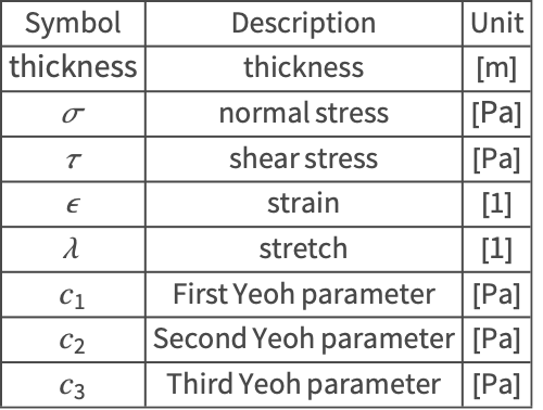
This model analyses the stress state of a coronary vessel under physiological conditions. The model makes use of a Yeoh hyperelastic material model with model parameters extracted from experimental procedures.
The coronary arteries are major blood vessels supplying blood to the heart. There are several diseases linked to the coronary arteries that can compromise an entire organism. A common type of heart disease is caused by plaque buildup in the wall of coronary arteries. Also, a coronary aneurism represents a dangerous pathology. It is defined as a dilatation of the coronary arteries in which the wall exceeds the normal diameter. These diseases are strongly linked to the wall of the arteries. The artery walls are an active structure that continuously remodels during the entire life of a human. It senses the bio-chemo-mechanical environment to guarantee homeostasis and the best blood supply to heart tissues [Mishani, 2021].

This figure shows the complexity reduction made from the anatomical structure of the coronary vessel to a simplified model that maintains mechanical properties of interest. The 2D structure is made up of three layers and symmetry constraints (only sliding in the edge-parallel direction) which allows representing the entire annulus.
The structure of the wall of an artery is complex. From a topological point of view, it consists of three different layers. The inner one, called tunica intima, is a layer made of epithelium and connective tissues with elastic fibers. The middle layer, the tunica media, is primarily made of smooth muscle cells and can regulate the arterial diameter due to local and central stimuli. The outer layer, the tunica adventitia, is made of connective tissue with collagen and elastic fibers. It links the artery to the surrounding structures.
Here a comparison between a triple-layered vessel and a homogenous one is presented. The three layers represent the tunica intima, media and adventitia, each one with different mechanical properties from the literature. Geometry is reduced to three concentric cylinders with a diameter representative of the anatomy of the main left coronary artery [Gholipour, 2018]. Furthermore, two different techniques to homogenize the vessel properties toward a homogeneous single-layer structure are implemented.
Four different modeling approaches are shown: First a simple analytical model is presented. Then, in a second model, the usage of the three-layer model with different material parameters in each layer to represent the tunica intima, media and adventitia is implemented. Then, the next two models represent simplified homogenizations. One of the homogenization approaches is to use the material parameters of the inner layer, the tunica intima layer, and in the second homogenization approach an area average of all three material layers is used.
In order to show the difference between a multilayer constitutive model and a single-layer model, an analysis of a uniaxial tensile traction test is performed. This is done by applying a stretch along a single direction, and it leads to ![]() and
and ![]() .
.
To enforce incompressibility, ![]() is set. It is then possible to express the first strain invariant
is set. It is then possible to express the first strain invariant ![]() with respect to the uniaxial stretch as:
with respect to the uniaxial stretch as:
And the Cauchy stress over the first principal direction reads:
intima = <| Subscript[, 1] -> 6.79 * 10 ^ 3, Subscript[, 2] -> 0.54 * 10 ^ 6, Subscript[, 3] -> -1.11 * 10 ^ 6|>;
media = <|Subscript[, 1] -> 6.52 * 10 ^ 3, Subscript[, 2] -> 4.89 * 10 ^ 2, Subscript[, 3] -> 9.26 * 10 ^ 3|>;
adventitia = <|Subscript[, 1] -> 8.27 * 10 ^ 3, Subscript[, 2] -> 1.20 * 10 ^ 4, Subscript[, 3] -> 0.52 * 10 ^ 6|>;Then it is possible to plot the material constitutive models as a bidimensional chart, strain vs. stress. With biological tissue, it is often useful to work with kPa, and a scale factor is introduced to rescale quantities.
scaleFactor = 10^-3;Uniaxial[c1_, c2_, c3_, λ_] := Block[{I1, dWdI, σunidirectional},
I1 = 2 / λ + λ^2;
dWdI = c1 + 2 * c2 * (I1 - 3) + 3 * c3 * (I1 - 3)^2;
σunidirectional = 2 * (λ^2 - 1 / λ) * dWdI;
scaleFactor * σunidirectional
];ListLinePlot[{
Table[{100 * (i - 1), Uniaxial[intima[Subscript[, 1]], intima[Subscript[, 2]], intima[Subscript[, 3]], i]}, {i, 1, 1.25, 0.01}],
Table[{100 * (i - 1), Uniaxial[media[Subscript[, 1]], media[Subscript[, 2]], media[Subscript[, 3]], i]}, {i, 1, 1.25, 0.01}],
Table[{100 * (i - 1), Uniaxial[adventitia[Subscript[, 1]], adventitia[Subscript[, 2]], adventitia[Subscript[, 3]], i]}, {i, 1, 1.25, 0.01}]
}, ...]Analytical Solution Approximation
This mechanical problem can be also reduced to a characteristic engineering problem where a cylinder or a sphere is subjected to an internal pressure ![]() . This is called a pressured vessel, and applications for it arise in many areas.
. This is called a pressured vessel, and applications for it arise in many areas.

This figure shows an ideal tube with length ![]() , thickness
, thickness ![]() and internal pressure
and internal pressure ![]() . It is possible to read circumferential stress
. It is possible to read circumferential stress ![]() and radial stress
and radial stress ![]() . Because of the open ends of the tube, the axial stress can be excluded.
. Because of the open ends of the tube, the axial stress can be excluded.
Here the analytical solution is shown for an inflated thickened-wall tube as an upper bound. This can be used to compare the stress state with a finite element solution. With biological tissues, the small strain hypothesis often fails, and this leads to several differences between this reduced analytical solution and the numerical one.
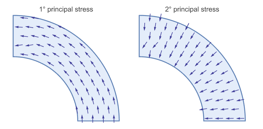
The first and the second principal stress directions are shown. The first principal stress ![]() is directed across the circumferential direction. The second principal stress
is directed across the circumferential direction. The second principal stress ![]() direction is along the radial direction.
direction is along the radial direction.
In the inflated tube, due to the internal pressure, the radial stress is related to this boundary pressure, at least on the internal side. It should also tend to zero on the external side, due to the absence of external force or pressure.
Furthermore, this cylinder shows the ratio ![]() , and this leads to the thick-walled vessels that could be calculated using the Lamé equation. Then it is possible to express the radial and tangential stress as:
, and this leads to the thick-walled vessels that could be calculated using the Lamé equation. Then it is possible to express the radial and tangential stress as:
with the internal pressure ![]() and the external pressure
and the external pressure ![]() .
.
The axial stress is close to zero, due to the absence of axial force or constraints.
parameters = <|Pin -> pressureMAX, Pout -> 0, a -> rin, b -> rout, A -> (Pin * a^2 - b^2 * Pout) / (b^2 - a^2), B -> (a^2  b^2 (Pin - Pout)) / (b^2 - a^2)|>;
σr[r_] := Evaluate[A - (B/r^2) //. parameters];
σθ[r_] := Evaluate[A + (B/r^2) //. parameters];diameter = scaleFactor 4.5;
rout = diameter / 2;
intima["Thickness"] = scaleFactor 0.23;
media["Thickness"] = scaleFactor 0.31;
adventitia["Thickness"] = scaleFactor 0.34;
rin = rout - (intima["Thickness"] + media["Thickness"] + adventitia["Thickness"] );
length = scaleFactor 16 ;
bloodPressure = Quantity[140, "mmHg"];
pressureMAX = QuantityMagnitude[UnitConvert[bloodPressure, "Pa"]];GraphicsRow[{
Plot[scaleFactor σr[scaleFactor r], {r, rin / scaleFactor, rout / scaleFactor}, ...],
Plot[scaleFactor σθ[scaleFactor r], {r, rin / scaleFactor, rout / scaleFactor}, ...]}]As it is possible to observe from the ![]() plot, the radial stress
plot, the radial stress ![]() is related to the boundary conditions. Indeed, the radial stress
is related to the boundary conditions. Indeed, the radial stress ![]() varies from the internal pressure
varies from the internal pressure ![]() on the lumen side of the vessel to
on the lumen side of the vessel to ![]() on the external side. The circumferential stress
on the external side. The circumferential stress ![]() is strongly related to the properties of the vascular tissue, and due to the high nonlinearity, large differences are present with respect to the following FEM analysis.
is strongly related to the properties of the vascular tissue, and due to the high nonlinearity, large differences are present with respect to the following FEM analysis.
Triple-Layered Model
The following FEM analysis represents the triple-layered model. It uses appropriate simplifications in geometry and constitutive models in order to reduce computational cost but still obtain accurate results. This relatively simplified analysis could be a starting point to investigate the mechanical environment of arteries and introduce further investigation, eventually with patient-specific geometries, to assess arteries' disease risk, development and progression [Holzapfel, 2018].
Needs["NDSolve`FEM`"]
$HistoryLength = 0;vars = {{u[x, y], v[x, y]}, {x, y}};Each layer is represented as a homogenous material described with the Yeoh hyperelastic model that can reproduce the nonlinearity present in the mechanical response of soft tissues such as biological tissue. Each layer uses different material parameters from literature [Gervaso, 2018].
The Yeoh hyperelastic constitutive model is a phenomenological model for representing the deformation of an isotropic, nearly incompressible, nonlinear elastic material such as rubber or biological tissues. The model is described by a strain energy density function represented as a power series of the strain invariant.
The Yeoh model implemented is a nearly incompressible model and can be used by specifying the "MaterialMoldel"->"Yeoh" in the parameter pars. The Yeoh model takes three parameters called "c1", "c2" and "c3" and it is described by a polynomial function representing the volumetric part of the strain energy density function ![]() :
:
For each layer, material parameters need to be specified. To make this process easy, a helper function is created to map the properties to each region.
DefineLayer[markerLayer_, layerName_] := With[
	{var1 = intima[layerName],
	var2 = media[layerName],
	var3 = adventitia[layerName],
	mrk1 = markerLayer[["Intima"]],
	mrk2 = markerLayer[["Media"]],
	mrk3 = markerLayer[["Adventitia"]]
	},
	Which[
	ElementMarker == mrk1, var1,
	ElementMarker == mrk2, var2,
	ElementMarker == mrk3, var3
	]
];markerLayer = <|"Intima" -> 1, "Media" -> 2, "Adventitia" -> 3|>;pars = <|"SolidMechanicsMaterialModel" -> "YeohIsotropic", "MassDensity" -> 1100,
Subscript[, 1] -> DefineLayer[markerLayer, Subscript[, 1]],
Subscript[, 2] -> DefineLayer[markerLayer, Subscript[, 2]],
Subscript[, 3] -> DefineLayer[markerLayer, Subscript[, 3]],
"Thickness" -> length,
"ConstitutiveStressMeasure" -> "SecondPiolaKirchhoff",
"EquilibriumStressMeasure" -> "FirstPiolaKirchhoff"|>;Also, see this note about how to set up computationally efficient PDE coefficients.
Mesh
In order to reduce the computational cost and better investigate the relationship between each layer, the analysis is reduced to a 2D section of the vessel. Furthermore, due to the rotational symmetry, only a quarter of the annulus is investigated, with corresponding symmetry conditions on the cutting edges.
bounds = Circle[{0, 0}, #, {0, π / 2}] & /@ {rin, rin + 0.23 / 1000 , rin + 0.23 / 1000  + 0.31 / 1000 , rout};
AppendTo[bounds, Line[{{0, rin}, {0, rout}}]];
AppendTo[bounds, Line[{{rin, 0}, {rout, 0}}]];
ru = RegionUnion[Flatten[bounds]];markerPoint = <|"Intima" -> (rin + (intima["Thickness"] / 2)) * {1, 0},
"Media" -> (rin + intima["Thickness"] + (media["Thickness"] / 2)) * {1, 0},
"Adventitia" -> (rout - (adventitia["Thickness"] / 2)) * {1, 0}|>;mesh = ToElementMesh[ru, {{-0.001, rout}, {-0.001, rout}}, "RegionMarker" -> {{markerPoint["Intima"], markerLayer["Intima"]}, {markerPoint["Media"], markerLayer["Media"]}, {markerPoint["Adventitia"], markerLayer["Adventitia"]}}, "MaxCellMeasure" -> 0.000000003];intima["Color"] = RGBColor[{ 204, 0, 0} / 255];
media["Color"] = RGBColor[{ 245, 245, 220} / 255];
adventitia["Color"] = RGBColor[{ 189, 116, 33} / 255];
mesh["Wireframe"["MeshElementStyle" -> {Directive[FaceForm[intima["Color"]]], Directive[FaceForm[media["Color"]]], Directive[FaceForm[adventitia["Color"]]]}]]It is important to guarantee a sufficient number of elements across the thickness of the layers. At least three layers of elements are needed for each region in order to estimate strain and stress without under-sampling the derivative. More elements would increase accuracy; however, the number of elements needs to be balanced with computational cost.
Show[mesh["Wireframe"["MeshElement" -> "BoundaryElements", "MeshElementIDStyle" -> Blue]],
	mesh["Wireframe"[ "MeshElementStyle" -> (Directive[EdgeForm[Gray], Opacity[0.5], FaceForm[#]]& /@ {intima["Color"], media["Color"], adventitia["Color"]})]],
	Graphics[{Red, Point[mesh["Coordinates"]]}],
	PlotRange -> {{0.99rin, 1.01rout}, {-0.01 rin, rin / 12}}, ImageSize -> Full]
Model Setup
For this model, two types of boundary conditions are needed: the symmetry conditions to model the reduced simulation domain and boundary conditions to model internal pressure. For more information on the symmetry condition, see the section on Displacement Constraints in the Solid Mechanics monograph. With regard to modeling the pressure, the goal is to set up a parametric solver with a parametric variable ![]() that is the imposed external load. The parameter
that is the imposed external load. The parameter ![]() allows the applied forces to slowly be increased, which is needed since the problem is too strongly nonlinear to solve in a single step. For more information on the solving of strongly nonlinear hyperelastic material models, see the Neo-Hookean model section in the Hyperelastic Solid Mechanics monograph.
allows the applied forces to slowly be increased, which is needed since the problem is too strongly nonlinear to solve in a single step. For more information on the solving of strongly nonlinear hyperelastic material models, see the Neo-Hookean model section in the Hyperelastic Solid Mechanics monograph.
The internal pressure needs to be specified as related to the physiological condition of the coronary arteries. A pressure of 140 mmHg [Ramanathan, 2005] is specified.
bloodPressure = Quantity[140, "mmHg"];
pressureMAX = QuantityMagnitude[UnitConvert[bloodPressure, "Pa"]];
The next step is to specify the positions where this pressure is applied.
Subscript[Γ, internal] = Annulus[{0, 0}, {rin - 0.1 * rin, rin + 0.1 * rin}, {0, π / 2}];
Subscript[Γ, predicate] = Refine[RegionMember[Subscript[Γ, internal], {x, y}], Assumptions -> {x, y}∈Reals];
The symmetry conditions apply at ![]() and
and ![]() , respectively and the displacement is set to 0 in the respective direction that the other direction left free to move. To avoid inaccuracies at the boundary, a tolerance is set.
, respectively and the displacement is set to 0 in the respective direction that the other direction left free to move. To avoid inaccuracies at the boundary, a tolerance is set.
boundaryTolerance = 10 ^ -9;pdeModel[vars_, pars_] := {SolidMechanicsPDEComponent[vars, pars] == SolidBoundaryLoadValue[Subscript[Γ, predicate], vars, pars, <|"Pressure" -> -p * {Indexed[NeumannBoundaryUnitNormal[{x, y}], 1], Indexed[NeumannBoundaryUnitNormal[{x, y}], 2]}|>],
SolidDisplacementCondition[x < boundaryTolerance, vars, pars, <|"Displacement" -> {0, None}|>],
SolidDisplacementCondition[y < boundaryTolerance, vars, pars, <|"Displacement" -> {None, 0}|>]
};pfun = ParametricNDSolveValue[pdeModel[vars, pars], vars[[1]], {x, y}∈mesh, p]Solution
Due to the high nonlinearity of the mechanical problem, the external load is slowly incremented.
nsteps = 80;
displacement = {0, 0};
AbsoluteTiming[Monitor[Do[
	pNew = step * pressureMAX / nsteps;
	displacement = pfun[pNew, "InitialSeeding" -> Thread[Equal[vars[[1]], displacement]]];
	, {step, 1, nsteps, 1}], step];]
When simulations run for a long time, it may make sense to store the obtained solution such that they are readily available later with out rerunning the simulation.
(*Export["displacement.mx",displacement]*)(*Import["displacement.mx"]*)Post-processing
After obtaining the solution, the data can be processed to investigate stress and strain fields in the domain of the sample.
Stress and strain can be extracted and plotted over both the original and the deformed mesh.
deformedMesh =
ElementMeshDeformation[mesh, displacement,
  "ScalingFactor" -> 1];
 Show[mesh["Wireframe"],   deformedMesh[  "Wireframe"[   "ElementMeshDirective" -> Directive[Opacity[0.2], Red]]]]
In order to analyze the stress and strain fields, they need to be extracted from the solution.
strains = SolidMechanicsStrain[vars, pars, displacement];GraphicsRow[ContourPlot[Extract[strains, #], {x, y}∈mesh,
...]& /@ {{1, 1}, {2, 2}} ]The strain fields along the ![]() and
and ![]() directions are reflected across the bisector
directions are reflected across the bisector ![]() at 45°. This is related to the rotational symmetry that this annulus implicitly shows. For this reason, another options is to plot the equivalent strain. The equivalent strain combines all strain components into a scalar, and as such is easier to grasp. The equivalent strain is used in the following comparison between homogenous and inhomogenous domains.
at 45°. This is related to the rotational symmetry that this annulus implicitly shows. For this reason, another options is to plot the equivalent strain. The equivalent strain combines all strain components into a scalar, and as such is easier to grasp. The equivalent strain is used in the following comparison between homogenous and inhomogenous domains.
equivalentStrain = EquivalentStrain[vars, pars, strains];ContourPlot[equivalentStrain, {x, y}∈mesh, ...]It is also interesting to investigate stress distribution across the thickness. The symmetric plots are also shown for the stress across the ![]() and
and ![]() directions. The Cauchy stress can be plotted, showing that it is higher on the inner layer than on the outer.
directions. The Cauchy stress can be plotted, showing that it is higher on the inner layer than on the outer.
cauchyStress = SolidMechanicsStress[vars, pars, strains, displacement] ;In order to represent the stress field, it is useful to use kPa units, so multiply by a conversion factor.
GraphicsRow[ContourPlot[Extract[scaleFactor cauchyStress, #1], {x, y}∈mesh, ...]& /@ {{1, 1}, {2, 2}} ]An alternative is to plot the von Mises stress, which represents an average across the different components of the stress. Indeed, its plot shows how the stress is higher on the inner layer side and slowly decreases from the inner layer to the outer one.
vonMisesStress = VonMisesStress[vars, pars, cauchyStress];vonMisesStressFunction = Head[vonMisesStress];
deformedVonMisesStress = ElementMeshInterpolation[deformedMesh, vonMisesStressFunction["ValuesOnGrid"]];minMaxMises = MinMax[vonMisesStressFunction["ValuesOnGrid"]];cp = ContourPlot[scaleFactor * deformedVonMisesStress[x, y], {x, y} ∈ deformedMesh, ...];
GraphicsRow[{Graphics[GeometricTransformation[cp[[1]], Table[RotationTransform[k Pi / 2], {k, 0, 4}]], ImageSize -> Medium], BarLegend[...]}]Also, an investigation of the principal stress direction is useful to understand the stress distribution.
{pricipalStressValues, pricipalStressVectors} = PDEModels`PrincipalEigensystem[vars, pars, cauchyStress];GraphicsRow[{
VectorPlot[pricipalStressVectors[[1]], {x, y}∈mesh, ...],
VectorPlot[pricipalStressVectors[[2]], {x, y}∈mesh, ...]}]The principal stresses are eigenvalues of the stress matrix and correspond to the diagonal stress values ![]() where the shear stress
where the shear stress ![]() is 0. For more information on the principal stresses, see the section on Principal Directions in the Solid Mechanics monograph. By plotting the principal stress direction, it is possible to show how the first one is directed tangentially to the annulus and is related to the stretch across the concentric circumferences. Moreover, the second principal direction appears across the radial direction and the second principal stress is mainly related to the internal boundary pressure and decreases to zero going outward. The following plots show the principal direction, while the stress values are shown in the following comparison or explained by the previous analytical solution.
is 0. For more information on the principal stresses, see the section on Principal Directions in the Solid Mechanics monograph. By plotting the principal stress direction, it is possible to show how the first one is directed tangentially to the annulus and is related to the stretch across the concentric circumferences. Moreover, the second principal direction appears across the radial direction and the second principal stress is mainly related to the internal boundary pressure and decreases to zero going outward. The following plots show the principal direction, while the stress values are shown in the following comparison or explained by the previous analytical solution.
Homogenized Models
The previous example made use of a three-layer model to describe the artery's wall. The question now is, How does a single-layer model compare to the three-layer model? In the following, two different homogenization approaches are shown. The first is using the material proprieties of the inner layer, the tunica intima, for all of the simulation domain. This is reasonable, especially in pathologies where an intima thickening is present, since in that case the tunica intima is the main load-carrying layer. The second approach uses a homogenization computed as an average of all three layers.
Homogenization with Intima Values
In order to homogenize the material properties, it is possible to use only the properties of the inner layer, the tunica intima. This is also reasonable following previous results showing higher stress in the intima that results in it being the main load-carrying layer.
parsIntimaValues = <|"SolidMechanicsMaterialModel" -> "YeohIsotropic", "MassDensity" -> 1100,
Subscript[, 1] -> intima[Subscript[, 1]],
Subscript[, 2] -> intima[Subscript[, 2]],
Subscript[, 3] -> intima[Subscript[, 3]],
"Thickness" -> length,
"ConstitutiveStressMeasure" -> "SecondPiolaKirchhoff",
"EquilibriumStressMeasure" -> "FirstPiolaKirchhoff"|>;pfunIntimaValues = ParametricNDSolveValue[pdeModel[vars, parsIntimaValues], vars[[1]], {x, y}∈mesh, p];nsteps = 80;
displacementIntimaValues = {0, 0};
AbsoluteTiming[Monitor[Do[
pNew = step * pressureMAX / nsteps;
displacementIntimaValues = pfunIntimaValues[pNew,
"InitialSeeding" ->
Thread[Equal[vars[[1]], displacementIntimaValues]]];
, {step, 1, nsteps, 1}],
step];]deformedMeshIntimaValues =
ElementMeshDeformation[mesh, displacementIntimaValues,
"ScalingFactor" -> 1];
strainsIntimaValues = SolidMechanicsStrain[vars, parsIntimaValues, displacementIntimaValues];
equivalentStrainIntimaValues = EquivalentStrain[vars, parsIntimaValues, strainsIntimaValues];
cauchyStressIntimaValues = SolidMechanicsStress[vars, parsIntimaValues, strainsIntimaValues, displacementIntimaValues] ;
vonMisesStressIntimaValues = VonMisesStress[vars, parsIntimaValues, cauchyStressIntimaValues];
vonMisesStressFunctionIntimaValues = Head[vonMisesStressIntimaValues];
deformedVonMisesStressIntimaValues = ElementMeshInterpolation[deformedMeshIntimaValues, vonMisesStressFunctionIntimaValues["ValuesOnGrid"]];Homogenization with Average Values
The second homogenization approach uses a mathematical average to homogenize the properties across the three layers into a single one.
averageProperties[coefficient_] := Round[NIntegrate[
	Which[
	ElementMarker == markerLayer["Intima"], intima[coefficient],
	ElementMarker == markerLayer["Media"], media[coefficient],
	ElementMarker == markerLayer["Adventitia"], adventitia[coefficient],
	True, 0
	], {x, y}∈mesh] / NIntegrate[1, {x, y}∈mesh]]
The usage of Round in the above helper function is to avoid numerical instabilities when converting the second Piola stress to a Cauchy stress. Since the average is only an approximation, the number is converted to its nearest integer. Since the integer itself is an exact number, the conversion to the Cauchy stress is less likely to run into trouble.
parsAverageValues = <|"SolidMechanicsMaterialModel" -> "YeohIsotropic", "MassDensity" -> 1100,
Subscript[, 1] -> averageProperties[Subscript[, 1]],
Subscript[, 2] -> averageProperties[Subscript[, 2]],
Subscript[, 3] -> averageProperties[Subscript[, 3]],
"Thickness" -> length,
"ConstitutiveStressMeasure" -> "SecondPiolaKirchhoff",
"EquilibriumStressMeasure" -> "FirstPiolaKirchhoff"|>;pfunAverageValues = ParametricNDSolveValue[pdeModel[vars, parsAverageValues], vars[[1]], {x, y}∈mesh, p];nsteps = 80;
displacementAverageValues = {0, 0};
AbsoluteTiming[Monitor[
Do[
pNew = step * pressureMAX / nsteps;
displacementAverageValues = pfunAverageValues[pNew, "InitialSeeding" -> Thread[Equal[vars[[1]], displacementAverageValues]]];
, {step, 1, nsteps, 1}]
, step];]deformedMeshAverageValues =
ElementMeshDeformation[mesh, displacementAverageValues,
"ScalingFactor" -> 1];
strainsAverageValues = SolidMechanicsStrain[vars, parsAverageValues, displacementAverageValues];
equivalentStrainAverageValues = EquivalentStrain[vars, parsAverageValues, strainsAverageValues];
cauchyStressAverageValues = SolidMechanicsStress[vars, parsAverageValues, strainsAverageValues, displacementAverageValues];
vonMisesStressAverageValues = VonMisesStress[vars, parsAverageValues, cauchyStressAverageValues];
vonMisesStressFunctionAverageValues = Head[vonMisesStressAverageValues];
deformedVonMisesStressAverageValues = ElementMeshInterpolation[deformedMeshAverageValues, vonMisesStressFunctionAverageValues["ValuesOnGrid"]];equivStrainMinMax = MinMax[Head[equivalentStrain]["ValuesOnGrid"]];
equivStrainMinMaxIntimaValues = MinMax[Head[equivalentStrainIntimaValues]["ValuesOnGrid"]];
equivStrainMinMaxAverageValues = MinMax[Head[equivalentStrainAverageValues]["ValuesOnGrid"]];Comparison
In this section, the three different FEM models are compared.
The layered structure shows more accurate results across the layers' interface. However, it requires more than 20 times the computational time of the homogenized ones. Depending on the interest of the simulation, it might be reasonable to use one model rather than the other; this requires evaluating the differences in stress and strain results to choose the optimal model.
globalEquivStrainMinMax = MinMax[{equivStrainMinMax, equivStrainMinMaxIntimaValues, equivStrainMinMaxAverageValues}];GraphicsColumn[{
GraphicsRow[{
Show[ContourPlot[equivalentStrain, {x, y}∈mesh, ...]],
Show[ContourPlot[equivalentStrainIntimaValues, {x, y}∈mesh, ...]],
Show[ContourPlot[equivalentStrainAverageValues, {x, y}∈mesh, ...]]
}],
BarLegend[{ColorData["TemperatureMap"][Rescale[#, globalEquivStrainMinMax]]&, globalEquivStrainMinMax}, ...]}, ImageSize -> Full]minMaxMisesIntimaValues = MinMax[vonMisesStressFunctionIntimaValues["ValuesOnGrid"]];
minMaxMisesAverageValues = MinMax[vonMisesStressFunctionAverageValues["ValuesOnGrid"]];globalvonMisesMinMax = scaleFactor * MinMax[{minMaxMises, minMaxMisesIntimaValues, minMaxMisesAverageValues}];GraphicsColumn[{
GraphicsRow[{Show[ContourPlot[scaleFactor deformedVonMisesStress[x, y], {x, y}∈deformedMesh, ...]],
Show[ContourPlot[scaleFactor deformedVonMisesStressIntimaValues[x, y], {x, y}∈deformedMeshIntimaValues, ...]], Show[ContourPlot[scaleFactor deformedVonMisesStressAverageValues[x, y], {x, y}∈deformedMeshAverageValues, ...]]}, ImageSize -> Large],
BarLegend[{ColorData["Rainbow"][Rescale[#, globalvonMisesMinMax]]&, globalvonMisesMinMax}, ...]}]The homogeneous and homogenized cases are closer together then the layered approach. The difference between the layered and the homogenized models is caused by the presence of an inner material boundary layer for the layered model, while no such layer exists in the homogenized models.
Then the stress measures are extracted across the thickness and plotted into an uniaxial chart. Due to the symmetry, these quantities remain the same for every radial direction.
BoxLayout[stress_] := Module[{rescale, color, colorFilling, myGraphs, radii, pointsToPlot}, (rescale = 10^3;
	color = {
	Directive[intima["Color"], Thickness[0.00001]],
	Directive[media["Color"], Thickness[0.00001]],
	Directive[adventitia["Color"], Thickness[0.00001]]
	};
	colorFilling = {Directive[Opacity[0.5], intima["Color"]],
	Directive[Opacity[0.5], media["Color"]],
	Directive[Opacity[0.5], adventitia["Color"]]
	};

	radii = rescale * {rin, rin + intima["Thickness"], rin + intima["Thickness"] + media["Thickness"], rout};

	pointsToPlot[MaxOrMinStress_] := Table[{{radii[[i]], MaxOrMinStress}, {radii[[i + 1]], MaxOrMinStress}}, {i, 1, Length[radii] - 1}];

	myGraphs = Show[ListLinePlot[pointsToPlot[Max[stress]], ...],
	ListLinePlot[pointsToPlot[Min[stress]], ...] ]
)];ExtractData[stress_, numberOfPoints_] := Table[{x / scaleFactor, scaleFactor * Head[stress][x, 10^-9]}, {x, rin, rout * 0.99, (rout - rin) / numberOfPoints}];numberOfPoints = 24;cs = {Blue, Orange, Purple};
misesIntimaValues = ExtractData[vonMisesStressIntimaValues, numberOfPoints];
misesAverageValues = ExtractData[vonMisesStressAverageValues, numberOfPoints];
mises = ExtractData[vonMisesStress, numberOfPoints];
Show[BoxLayout[mises],
ListLinePlot[{misesIntimaValues, misesAverageValues, mises}, PlotStyle -> cs, PlotLegends -> {"Intima values", "Averaged values", "Triple-layered"}], ...]σ11 = ExtractData[cauchyStress[[1, 1]], numberOfPoints];
σ22 = ExtractData[cauchyStress[[2, 2]], numberOfPoints];σ11IntimaValues = ExtractData[cauchyStressIntimaValues[[1, 1]], numberOfPoints];
σ22IntimaValues = ExtractData[cauchyStressIntimaValues[[2, 2]], numberOfPoints];σ11AverageValues = ExtractData[cauchyStressAverageValues[[1, 1]], numberOfPoints];
σ22AverageValues = ExtractData[cauchyStressAverageValues[[2, 2]], numberOfPoints];Show[BoxLayout[σ11AverageValues], ListLinePlot[{σ11IntimaValues, σ11AverageValues, σ11}, ...], ...]The first principal stress is related to the stretch in the tangential direction. Indeed, the different models show different strain distributions. These differences are what cause differences in the von Mises stress across the different models, as can be seen from the figure.
Show[BoxLayout[σ22], ListLinePlot[{σ22IntimaValues, σ22AverageValues, σ22}, ...], ...]The second principal stress is similar between each model; indeed, this is the stress in the radial direction and in the internal side has to contrast the internal pressure of the boundary value problem (equilibrium law). Then it should go to zero across the thickness, due to the absence of external pressure.
It is also interesting that across the interface between the intima and the media layer, the stress distribution coincides between the three models. Furthermore, the triple-layered model shows a major load-carrying role for the intima layer, with lower stress in the other layers. In the homogeneous and homogenized cases, the stress field continuously decreases from the internal side to the external one.
Nomenclature
References
1. A. Gholipour, M. H. Ghayesh, A. Zander and R. Mahajan (2018). "Three-Dimensional Biomechanics of Coronary Arteries." International Journal of Engineering Science, vol. 130, pp. 93–114, https://doi.org/10.1016/j.ijengsci.2018.03.002
2. S. Mishani, H. Belhoul-Fakir, C. Lagat, S. Jansen, B. Evans and M. Lawrence-Brown, (2021). "Stress Distribution in the Walls of Major Arteries: Implications for Atherogenesis." Quantitative Imaging in Medicine and Surgery, vol. 11, https://qims.amegroups.com/article/view/68560
3. G. A. Holzapfel and R. W. Ogden (2018). "Biomechanical Relevance of the Microstructure in Artery Walls with a Focus on Passive and Active Components." American Journal of Physiology-Heart and Circulatory Physiology, vol. 315, https://doi.org/10.1152/ajpheart.00117.2018
4. F. Gervaso, C. Capelli, L. Petrini, S. Lattanzio, L. Di Virgilio and F. Migliavacca (2016). "On the Effects of Different Strategies in Modelling Balloon-Expandable Stenting by Means of Finite Element Method." Journal of Biomechanics, vol. 41, pp. 1206–1212, https://doi.org/10.1016/j.jbiomech.2008.01.027
5. T. Ramanathan and H. Skinner, (2005). "Coronary Blood Flow." Continuing Education in Anaesthesia Critical Care & Pain, vol. 5, pp. 1743–1816, https://doi.org/10.1093/bjaceaccp/mki012