Biaxial Tensile Test of Hyperelastic Tissue

Introduction

Biaxial tensile testing is an experimental technique to characterize materials. For this purpose a rectangular material specimen is perforated with holes that act as anchors for hooks. The hooks will be pulled apart and both the forces applied and the resulting displacements measured. An illustration of a specimen pulled with a typical number of hooks is shown below.

Highlighted in red is the symmetry of the setup, which we will exploit later in order to reduce computational complexity.

The experimental tools for biaxial tensile testing provide a high measurement resolution and, additionally, the possibility to measure in orthogonal directions which allows to characterize anisotropic material. The results from a biaxial tension test can then be used to calibrate a hyperelastic material model. While biaxial tensile testing is not a new technique, applying biaxial tensile testing to biological material is [Fehervary,2016]

The following notebook implements a finite element simulation of a biaxial test. Biaxial tests are generally used to show anisotropic behavior. To keep things simple, this example uses an isotropic Neo-Hookean model. We make use of material parameters for vascular tissue obtained from literature [Karimi,2013]. This allows us to compare the computational results with experimental results [Zemanek,2008].

2D FEM model

For the model we use a stationary 2D plane stress model form.

We make use of a Neo-Hookean material model, with parameters from literature.

Geometry

Since the specimen and the positioning of the hooks is symmetric, it is sufficient to to model a quarter of the specimen using two fold symmetry. We start by specifying the length and thickness of the reduced simulation domain and specify the hole radius.

Model setup

For this model, two types of boundary conditions are needed. The symmetry conditions to model the reduced simulation domain and boundary conditions to model the pulling of the hooks. For modeling the pulling of the hooks, the goal is to set up a parametric solver with a parametric variable that is a prescribed displacement. The parameter allows us to slowly increase the applied forces, which is needed since the problem is too strongly nonlinear to solve in a single step. For more information see the sections on strongly nonlinear Hypoelastic models and on Displacement Conditions in the Solid Mechanics monograph.

First, we look at the symmetry condition. The symmetry conditions apply at and , respectively and the displacement is set to 0 in the respective direction which the other direction left free to move.

For the pulling of the hooks we also use displacement conditions. We specify a total displacement of up to 40% and to set the boundary conditions for that.

Specify the total displacement, the maximal value of :

The next step is to specify the positions where these hooks are placed. We assume that the hooks are rigid and the pulling happens in that half of the boundary of the holes in which the force is acting. To make this easy, we select a rectangular region around the respective holes.

To make use of these rectangular regions we use RegionMember to convert them to predicates suitable for the solid mechanics boundary conditions. The result from RegionMember includes constraints that the numbers must be real. In the finite element simulation the mesh coordinates are always real and we can remove the constraint by using Refine.

Since DirichletCondition are only applied at boundaries nodes of the mesh, these predicates now correspond to the semicircles that are the intersection of the blue circles and the coloured rectangles, as highlighted in red and green in the figure above.

Note, the value of applied displacement is given via the parameter . Also note that for the right predicate we use a displacement that is 0.8 times that for the top displacement. For biaxial tension testing various force configurations are used to measure the material characteristics. Here, we have arbitrarily chosen a factor of 0.8 between the two directions.

Solution

To solve the PDEs with the strong non-linearity of the hyperelasticity we can use the parametric solver by gradually increasing the displacement using a sufficient number of steps. Furthermore, for each step we can extract the stress-strain relation to obtain the final curve describing the tensile test experimental procedure. To extract stress and strain we can use the averaged Cauchy stress.

To reduce the simulation time and memory usage, the strain, stress and stress-strain curve are only computed every 10th step.

Post processing

After obtaining the solution we can process the data to investigate stress and strain fields in the domain of the sample.

First of all we can observe the stress-strain relation obtained from each step of the parametric solver. We can also compare this curve with experimental data [Zemanek,2008].

We can observe the effect of traction done by the hooks in both directions. We can plot the Cauchy stress over the stretch, related to the engineering strain as . The hyperelastic material shows a high deformation, up to 40%, and we can see a good correspondence with the experimental data. The model is very good up to 20% of strain however at high deformation starts to deviate from the experimental data. Nevertheless it remains a good model to describe this vascular tissue and in order to better fit the data the material parameters could be optimized, which is outside the scope of this model.

Next, we can extract stress and strain and plot them over both the original and the deformed mesh.

In order to create an animation of deformation process, we first compute the bounds of the final deformation. These bounds will then be used as PlotRange bounds such that all animation frames use the same plot area.

A note about the quality of the visualization: To get high fidelity visualizations comment out the call to Rasterize above.

In order to analyze stress and strain field we need to extract these fields from the solution, then we can plot them.

We can see how the sample is stretched. The deformation is more intense in the top holes, as we can expect from boundary conditions and observe from the central plot. The shear strain looks almost symmetric, however, it is slightly unbalanced in the -direction, due to the greater deformation.

In order to represent the stress field it is useful to use MPa units, so we multiply by a conversion factor.

We can see the normal stress along the -direction and -direction that reflects the tensile state due to the boundary conditions. It is focused around the area of the holes and appears to be higher in the -direction.

The von Mises stress is a scalar value used to represent the stress state in the material. It is calculated by taking a weighted average of the different components of the stress tensor, as expressed in the Solid Mechanics monograph.

We can see that the von Mises stress field is generally homogenous in the tissue and the higher stresses appear near to the holes. This is related to the traction boundary conditions which stretch the sample from the holes.

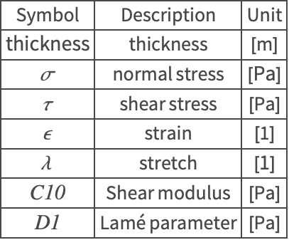
Nomenclature

References

1.  H. Fehervary, M. Smoljkić, J. Vander Sloten, and N. Famaey, (2016). Planar biaxial testing of soft biological tissue using rakes: A critical analysis of protocol and fitting process. Journal of the Mechanical Behavior of Biomedical Materials, vol. 61, pp. 135–151, https://doi.org/10.1016/j.jmbbm.2016.01.011

2.  Karimi A, Navidbakhsh M, Faghihi S, Shojaei A, Hassani K. A finite element investigation on plaque vulnerability in realistic healthy and atherosclerotic human coronary arteries. Proceedings of the Institution of Mechanical Engineers, Part H: Journal of Engineering in Medicine. 2013;227(2):148-161, https://doi.org/10.1177/0954411912461239

3.  Zemánek, Miroslav & Bursa, Jiri & Děták, Michal. (2008). Biaxial Tension Tests with Soft Tissues of Arterial Wall. 16, https://www.researchgate.net/publication/41842810_Biaxial_Tension_Tests_with_Soft_Tissues_of_Arterial_Wal