Thermal and Structural Analysis of a Disc Brake
| Introduction | 2D Axisymmetric Structural Mechanics Model |
| Multiphysics Model | Model Extensions |
| Axisymmetric Heat Transfer Equation | Nomenclature |
| Domain | References |
| 2D Axisymmetric Heat Transfer Model |
Introduction
A braking system is generally composed of a brake disc and two brake pads. When braking, the brake pads exert pressure on the disc to decelerate it. In this process, there is a transformation of mechanical energy to thermal energy due to the friction between the pads and the disc. This energy is then dissipated in the material of the disc, causing a change in the temperature distribution ![]() in
in ![]() . This nonuniform temperature distribution in the brake disc induces thermal stresses due to thermal expansion [Adamowicz,2015].
. This nonuniform temperature distribution in the brake disc induces thermal stresses due to thermal expansion [Adamowicz,2015].
This notebook demonstrates a transient thermal analysis to calculate the temperature distribution caused by braking, and a quasi-static thermal stress analysis. The geometry of the disc and brake pads is mostly rotationally symmetric, and an axisymmetric analysis will be shown. The model shown is a simplified disc brake that has brake pads all around, based on [Adamowicz,2015]. The rotationally symmetric assumption is warranted by the fact that the disc rotates quickly, compared to the size of the pads.
Revolving the black rectangular region, which is the cross section through the brake disc, around the ![]() axis, the axis of revolution, arrives at the 3D model geometry as seen in the figure below.
axis, the axis of revolution, arrives at the 3D model geometry as seen in the figure below.

Needs["NDSolve`FEM`"]Multiphysics Model
There are two physical domains involved in this application: the heat transfer model and the structural mechanics model. The coupling between the two models is one-way: the disc deformation depends on the temperature only. In this model, it is assumed that the influence of the deformed disc on the temperature field is small and thus it is not considered.
This type of problem is considered a sequential multiphysics model and will be solved in two steps.
First, the heat transfer model is solved to get the temperature distribution ![]() of the disc. Then, the structural mechanics model is constructed and the thermal stresses are computed at several solution times, using the temperature distribution previously computed.
of the disc. Then, the structural mechanics model is constructed and the thermal stresses are computed at several solution times, using the temperature distribution previously computed.
Axisymmetric Heat Transfer Equation
The phenomenon of heat transfer is described by the heat equation, but in this example can be described by a special case of the heat equation: the axisymmetric form. This can be done because the domain and the boundary conditions are rotationally symmetric about the ![]() axis. Using an axisymmetric model has the advantage that the computational cost in both time and memory is much less than in the case of solving a 3D heat transfer problem.
axis. Using an axisymmetric model has the advantage that the computational cost in both time and memory is much less than in the case of solving a 3D heat transfer problem.
The axisymmetric heat transfer equation is given as:
where ![]() is the mass density in
is the mass density in ![]() ,
, ![]() is the specific heat capacity in
is the specific heat capacity in ![]() , and
, and ![]() is the thermal conductivity in
is the thermal conductivity in ![]() .
.
The axisymmetric heat equation uses a truncated cylindrical coordinate system in 2D with independent variables ![]() instead of the cylindrical coordinates
instead of the cylindrical coordinates ![]() . The cylindrical coordinate variable
. The cylindrical coordinate variable ![]() disappears because the system is rotationally symmetric about the
disappears because the system is rotationally symmetric about the ![]() axis.
axis.
More information on the axisymmetric heat equation is given in the section "Special Cases of the Heat Equation" in the Heat Transfer overview monograph.
Axisymmetric Structural Mechanics Model
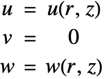
Just as in the heat transfer model, an axisymmetric structural solid mechanics simulation can be performed, because the 3D solid is rotationally symmetric about the ![]() axis. As in the 3D Cartesian model, the displacements are still called
axis. As in the 3D Cartesian model, the displacements are still called ![]() ,
, ![]() and
and ![]() , but now
, but now ![]() is the displacement in the radial direction
is the displacement in the radial direction ![]() ,
, ![]() the displacement in the angular direction
the displacement in the angular direction ![]() , and
, and ![]() the displacement in the axial direction
the displacement in the axial direction ![]() . The assumption for the axisymmetric model is that there is no displacement in the
. The assumption for the axisymmetric model is that there is no displacement in the ![]() direction. This means that
direction. This means that ![]() , and that
, and that ![]() and
and ![]() are independent of
are independent of ![]() , arriving at a truncated cylindrical coordinate system in 2D with independent variables
, arriving at a truncated cylindrical coordinate system in 2D with independent variables ![]() .
.
Therefore, the constitutive equation can be given as:
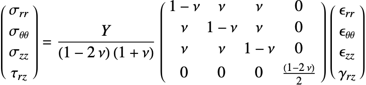
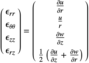
where the strain vector is given by:
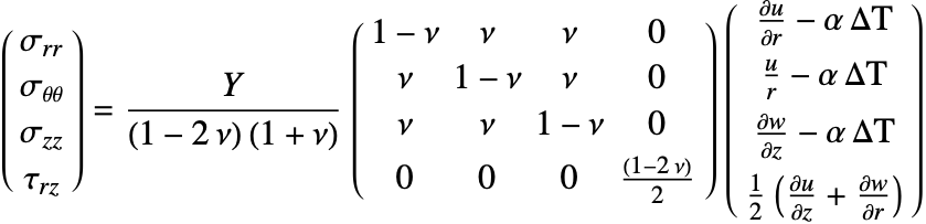
Now, to consider the thermal effects, an initial strain ![]() is included in the constitutive equation as follows:
is included in the constitutive equation as follows:
In this case, ![]() represents a thermal strain, which is given by:
represents a thermal strain, which is given by:
where ![]() is the constant coefficient of linear thermal expansion (CLTE), measured in
is the constant coefficient of linear thermal expansion (CLTE), measured in ![]() ,
, ![]() is the temperature of the body in
is the temperature of the body in ![]() , and
, and ![]() is the reference temperature, also in
is the reference temperature, also in ![]() , at which there is no thermal strain in the body. A more detailed explanation can be found in the linear thermal expansion section of the Solid Mechanics tutorial.
, at which there is no thermal strain in the body. A more detailed explanation can be found in the linear thermal expansion section of the Solid Mechanics tutorial.
The axisymmetric case additionally requires that the equilibrium equations be adapted to the cylindrical coordinate system. More information on the axisymmetric solid mechanics approximation is given in the Axisymmetric Solid Mechanics section.
Domain
The domain of analysis in this case is an axially symmetric geometry, also known as body of revolution. The sketch below shows the simulation domain, which is a rectangular region (disc) and one of the two brake pads.

In the following, all length scales are given in meters ![]() . The simulation setup consists of a disc and a pad, and there are various symmetries that are exploited. One is the rotational symmetry around the
. The simulation setup consists of a disc and a pad, and there are various symmetries that are exploited. One is the rotational symmetry around the ![]() axis, which allows the simulation domain to be reduced to a rectangular region corresponding to the axisymmetric section of the annular disc. A second symmetry is indicated by the cut line though the disc. Normally, a brake system has a disc and two brake pads acting on the disc, one on either side. Due to the second symmetry, it is possible to halve the disc thickness and only model one pad. The equation is then solved in the reduced disc, and the pad is modeled as a boundary condition.
axis, which allows the simulation domain to be reduced to a rectangular region corresponding to the axisymmetric section of the annular disc. A second symmetry is indicated by the cut line though the disc. Normally, a brake system has a disc and two brake pads acting on the disc, one on either side. Due to the second symmetry, it is possible to halve the disc thickness and only model one pad. The equation is then solved in the reduced disc, and the pad is modeled as a boundary condition.
In the following, all length scales are given in meters ![]() . The example models half the thickness of the disc
. The example models half the thickness of the disc ![]() , indicated by the dashed cut line, and the effect of one brake pad Pad 1 through the boundary condition. The geometry is described by the inner disc radius
, indicated by the dashed cut line, and the effect of one brake pad Pad 1 through the boundary condition. The geometry is described by the inner disc radius ![]() and outer disc radius
and outer disc radius ![]() , the inner radius
, the inner radius ![]() and outer radius
and outer radius ![]() of the pad, the half thickness of the disc
of the pad, the half thickness of the disc ![]() , and the thickness of the pad
, and the thickness of the pad ![]() .
.
In a typical brake system, the outer radius of the disc ![]() is larger than the outer radius of the pad
is larger than the outer radius of the pad ![]() , but to stay consistent with [Adamowicz,2015], both outer radii were made equal. The first sketch also shows in which region the heat flow
, but to stay consistent with [Adamowicz,2015], both outer radii were made equal. The first sketch also shows in which region the heat flow ![]() takes place.
takes place.
Subscript[r, disc] = 0.066;
Subscript[r, pad] = 0.0765;
Subscript[R, disc] = Subscript[R, pad] = 0.1135;
Subscript[δ, disc] = 0.0055;
Subscript[δ, pad] = 0.01;
To make use of boundary markers, the boundary mesh is created manually, using ToBoundaryMesh. These markers can then be used to set up the boundary conditions on the geometry. Using markers can be simpler than specifying the formula for each boundary. This is explained further in the section "Markers" in the "Element Mesh Generation" tutorial.
bmesh = ToBoundaryMesh[
	"Coordinates" -> {{Subscript[r, disc], -Subscript[δ, disc] }, {Subscript[R, disc], -Subscript[δ, disc] }, {Subscript[R, disc], 0}, {Subscript[r, pad], 0}, {Subscript[r, disc], 0}},
"BoundaryElements" -> {LineElement[{{1, 2}, {2, 3}, {3, 4}, {4, 5}, {5, 1}}, {1, 2, 3, 4, 5}]}];bmesh["Wireframe"["MeshElementMarkerStyle" -> Black, "MeshElementStyle" -> {Blue, Red, Green, Yellow, Purple}]]Each of the marked edges will be used to position boundary conditions discussed later.
mesh = ToElementMesh[bmesh, "MaxCellMeasure" -> 1*^-7];A max cell measure value was applied to the mesh to get a more accurate result.
2D Axisymmetric Heat Transfer Model
In the following section, the heat transfer model will be solved to simulate the temperature field ![]() of the disc.
of the disc.
Parameters Setup
In a next step the material parameters and the 2D axisymmetric transient heat transfer equation are set up. According to [Adamowicz,2015], the disc is made of cast iron ChNMKh and the pad is made out of cermet FMC-11. The mass density ![]() in
in ![]() , the specific heat capacity
, the specific heat capacity ![]() in
in ![]() and the thermal conductivity
and the thermal conductivity ![]() in
in ![]() of the disc will be defined.
of the disc will be defined.
Later, when the boundary conditions are specified, it is more convenient to be able to access the parameter values directly than through their property names, and thus the definition is split.
pars = <||>;
pars["MassDensity"] = Subscript[ρ, disc];
pars["ThermalConductivity"] = Subscript[k, disc] * IdentityMatrix[2];
pars["SpecificHeatCapacity"] = Subscript[Cp, disc];
Next, the actual values are defined.
pars[Subscript[ρ, disc]] = 7100;
pars[Subscript[k, disc]] = 51;
pars[Subscript[Cp, disc]] = 498.826;Subscript[T, 0] = 293.15;
ic = {T[0, r, z] == Subscript[T, 0]};The HeatTransferPDEComponent function can produce the axisymmetric form of the heat transfer equation. To do so, the parameter "RegionSymmetry" is set to "Axisymmetric".
vars = {T[t, r, z], t, {r, z}};
pars["RegionSymmetry"] = "Axisymmetric";
op = HeatTransferPDEComponent[vars, pars]
Boundary Conditions
As mentioned above, the equation is only solved on the disc, while the pad is modeled as a boundary condition, so there are two boundary conditions involved in this model that need to be defined.
One is a heat flux boundary condition to account for the heat flux that the pad generates in the region where it is placed. The heat flux is active at the boundary element marker 3, that is, from the inner radius of the pad ![]() to the outer radius of the pad
to the outer radius of the pad ![]() . The heat flux is given by a function
. The heat flux is given by a function ![]() , which is the heat flux generated during a single braking process from a constant initial angular speed to a standstill, described in [Adamowicz,2015].
, which is the heat flux generated during a single braking process from a constant initial angular speed to a standstill, described in [Adamowicz,2015].
The second boundary condition is a heat insulation condition and is active on the boundary parts marked with boundary element markers 1, 2, 4 and 5. A HeatInsulationValue produces a Neumann 0 value. As these are the natural default boundary conditions, they can be left out.
Apart from that, the yellow boundary with element marker 4 will be used differently in a later section where the model is extended further.
pars[Subscript[k, pad]] = 34.3;pars[Subscript[ρ, pad]] = 4700;pars[Subscript[Cp, pad]] = 499.854;pars["PadFrictionCoefficient"] = 0.5;pars["PadAngularVelocity"] = 88.464;pars["PadContactPressure"] = (1.47*^6) * (64.5 / 360);qflux[{t_, tend_}, {r_, z_}, pars_] := Module[
{alphap, kp, ρp, Cpp, f, omega0, p0, omegat, eta, q, kd, ρd, Cpd, qd},
kd = pars[Subscript[k, disc]];
ρd = pars[Subscript[ρ, disc]];
Cpd = pars[Subscript[Cp, disc]];
kp = pars[Subscript[k, pad]];
ρp = pars[Subscript[ρ, pad]];
Cpp = pars[Subscript[Cp, pad]];
f = pars["PadFrictionCoefficient"];
omega0 = pars["PadAngularVelocity"];
p0 = pars["PadContactPressure"];
omegat = omega0 * (1 - (t / tend));
eta = Sqrt[kd * ρd * Cpd] / (Sqrt[kd * ρd * Cpd] + Sqrt[kp * ρp * Cpp]);
qd = eta * f * omegat * r * p0;
Return [qd]
]Subscript[Γ, flux] = HeatFluxValue[ElementMarker == 3, vars, pars, <|"HeatFlux" -> qflux[{t, tend}, {r, z}, pars]|>];Model Evaluation
What remains is to compute the numeric solution of the PDE with NDSolveValue.
tend = 3.96;measure = AbsoluteTiming[MaxMemoryUsed[Tfun = NDSolveValue[{op == Subscript[Γ, flux], ic}, T, {t, 0, tend}, {r, z}∈mesh]] / (1024. ^ 2)];
Print["Time -> ", measure[[1]], "
Memory -> ", measure[[2]]];Post-processing and Visualization
Plot the temperature changes on the contact surface of the disc ![]() during braking at key radial locations: at the inner and outer radius of disc and pad.
during braking at key radial locations: at the inner and outer radius of disc and pad.
Plot[{Tfun[t, Subscript[R, disc], 0], Tfun[t, Subscript[r, pad], 0], Tfun[t, Subscript[r, disc], 0]}, {t, 0, tend}, ...]The resulting data is comparable to the Fig. 2. shown in [Adamowicz,2015].
frames = Table[Labeled[Legended[ContourPlot[Tfun[t, r, z], {r, z}∈ mesh, ...], BarLegend[...]], Text[...]], {t, 0, tend, 0.1}];
frames = Rasterize[#1, "Image", ImageResolution -> 80]& /@ frames;
ListAnimate[frames, SaveDefinitions -> True]
See this note about improving the visual quality of the animation.
Show[Legended[RegionPlot3D[Subscript[r, disc] ^ 2 <= x ^ 2 + y ^ 2 <= Subscript[R, disc] ^ 2, {x, -Subscript[R, disc] * 2, Subscript[R, disc] * 2}, {y, -Subscript[R, disc] * 2, Subscript[R, disc] * 2}, {z, 0, Subscript[δ, disc]}, ...], BarLegend[...]], Graphics3D[{...}], PlotRange -> {{0.04, 0.12}, {-0.05, 0.05}, All}]To visualize the full 3D solution from the axisymmetric model, one can apply the interpolating function to visualize the data in a 3D domain. In other words, do a revolution plot of the data.
Use RegionPlot3D to make a plot showing the three-dimensional region in which pred is the equation of the annular disc.
Legended[RegionPlot3D[Subscript[r, disc] ^ 2 <= x ^ 2 + y ^ 2 <= Subscript[R, disc] ^ 2, {x, -Subscript[R, disc] * 2, Subscript[R, disc] * 2}, {y, -Subscript[R, disc] * 2, Subscript[R, disc] * 2}, {z, -Subscript[δ, disc], 0}, ...], BarLegend[...]]2D Axisymmetric Structural Mechanics Model
In the following section, the structural mechanics model is constructed and solved to show the thermally induced stresses.
Parameters Setup
First, the missing material parameters and the 2D axisymmetric solid mechanics PDE terms are set up. The Young modulus ![]() in
in ![]() , the Poisson ratio
, the Poisson ratio ![]() and the thermal expansion coefficient
and the thermal expansion coefficient ![]() in
in ![]() of the disc will be defined.
of the disc will be defined.
pars["YoungModulus"] = 99.97*^9;
pars["PoissonRatio"] = 0.29;
pars["ThermalExpansion"] = 1.08*^-5;pars["ThermalStrainReferenceTemperature"] = Subscript[T, 0];
pars["ThermalStrainTemperature"] = T[t, r, z];The SolidMechanicsPDEComponent function can produce the axisymmetric form of the solid mechanics PDE terms. To do so, the parameter "RegionSymmetry" in pars needs to be set to "Axisymmetric", which was already done above.
pars["RegionSymmetry"]Here, the axisymmetric case is treated like a 3D setup. To make use of this, the dependent variable ![]() is set to 0 in the dependent variable setup. The actual computation, however, will still be done in 2D. This has several advantages. First, the returned displacement will also have
is set to 0 in the dependent variable setup. The actual computation, however, will still be done in 2D. This has several advantages. First, the returned displacement will also have ![]() set, and secondly, both stress and strain will have the
set, and secondly, both stress and strain will have the ![]() components set. Vector-valued parameters are now specified as three-component vectors.
components set. Vector-valued parameters are now specified as three-component vectors.
varsSM = {{u[r, z], 0, w[r, z]}, {r, θ, z}};
QuasiStructuralModel = SolidMechanicsPDEComponent[varsSM, pars];
Boundary Conditions
According to [Adamowicz,2015], the only constraint that the disc has is a zero displacement in the ![]() direction at the disc bottom. Nevertheless, this constraint is insufficient to prevent rigid body motion, as mentioned here. A constraint for the displacement
direction at the disc bottom. Nevertheless, this constraint is insufficient to prevent rigid body motion, as mentioned here. A constraint for the displacement ![]() should be specified.
should be specified.
To prevent rigid body motion, a zero displacement is specified in the ![]() direction at the disc left edge.
direction at the disc left edge.
Subscript[Γ, roller] = SolidDisplacementCondition[ElementMarker == 1, varsSM, pars, <|"Displacement" -> {None, None, 0}|>];Subscript[Γ, roller2] = SolidDisplacementCondition[ElementMarker == 5 , varsSM, pars, <|"Displacement" -> {0, None, None}|>] ;It should be mentioned that mechanical loads, like gravity, in the disc are not taken into account.
Model Evaluation
In this model, a quasi-static approach is taken to solve the structural solid mechanics model as in [Adamowicz,2015]. Quasi-static means one solves the steady-state solid mechanics equation at a desired time of the temperature distribution solution. This can done repetitively at different times.
One might be inclined to use ParametricNDSolve for this task, but in current versions of the Wolfram Language, parametric functions cannot take nonconstant arguments. This means that one needs to revert back to use NDSolve and replace the parameter with the interpolating function manually.
tList = {0.1, 0.2, 1, 2, 3, tend};n = Length[tList];It is computationally more efficient to create a new interpolating function at each point in time of interest. This is explained in more detail here.
TempFun[t_] := ElementMeshInterpolation[{mesh}, Function[{r, z}, Tfun[t, r, z]]@@@mesh["Coordinates"]];TfunList = TempFun[#][r, z]& /@ tList;pdeList = Table[{QuasiStructuralModel == {0, 0}, Subscript[Γ, roller], Subscript[Γ, roller2]} /. T[t, r, z] -> TfunList[[i]], {i, n}];measure = AbsoluteTiming[MaxMemoryUsed[Monitor[displacementList = Table[NDSolveValue[pdeList[[i]], varsSM[[1]], {r, z} ∈ mesh
], {i, n}], Row[{"t = ", CForm[tList[[i]]]}]]] / (1024. ^ 2)];
Print["Time -> ", measure[[1]], "
Memory -> ", measure[[2]]];Post-processing and Visualization
The objective of this simulation is to see the thermal stresses induced by the nonuniform temperature distribution. To obtain the thermal stresses, the strains first need to be computed from the displacements, and then the stresses can be recovered from the strains.
strainList = SolidMechanicsStrain[varsSM, pars, #]& /@ displacementList;stressList = Table[SolidMechanicsStress[varsSM, pars /. T[t, r, z] -> TfunList[[i]], strainList[[i]], displacementList[[i]]], {i, n}];sRangeList = Table[MinMax[Head[stressList[[i, 1, 1]]]["ValuesOnGrid"]], {i, n}];
GraphicsColumn[Table[ContourPlot[stressList[[i, 1, 1]], {r, z}∈ mesh, ...], {i, n}], ImageSize -> Full]It is also possible to compute the von Mises stress.
vonMisesStressList = VonMisesStress[varsSM, pars, #]& /@ stressList;vonMisesStressFunctionList = Head /@ vonMisesStressList ;Table[MinMax[vonMisesStressFunctionList[[i]]["ValuesOnGrid"]], {i, n}]ContourPlot[Head[vonMisesStressList[[n]]][r, z], {r, z}∈ mesh, ...]Finally, a visualization is generated to show how much deformation occurred in the disc compared to the original one.
deformedMesh = ElementMeshDeformation[mesh, {displacementList[[n, 1]], displacementList[[n, 3]]}, "ScalingFactor" -> 10];Show[mesh["Wireframe"["MeshElement" -> "BoundaryElements"]],
deformedMesh["Wireframe"["MeshElement" -> "BoundaryElements", "MeshElementStyle" -> Red]]]It should be noted that the results shown here differ from those of [Adamowicz,2015] because of the additional constraint to prevent rigid body motion in the radial direction that was added on the left edge of the disc.
Model Extensions
The previous section introduced a simple disc brake PDE model. In this section, the model is enhanced in two ways, to allow for more realistic simulations. First, the material parameters will be temperature dependent and second, the thermal heat dissipation of the disc will be modeled by applying thermal convection and thermal radiation on the boundary.
Nonlinear Material Parameters
Depending on the carbon content in the disc, both the density and the thermal conductivity drop with increased temperature, while the heat capacity increases with temperature. For all properties, a simple linear model is used. For this, simple data points are created and a linear fit to the material data is found. An alternative approach is to use an interpolating function as the material coefficients. This will also work; the find fit approach has the advantage that a time integration will be faster than when using the interpolating function approach, simply because the evaluation of the symbolic find fit model is more efficient than the lookup and interpolation in the interpolating function. Of course, a higher-order model for the fit could be used.
model = T[t, r, z] * a + b;data = {{273, 51}, {573, 49}};
linearThermalConductivityFit = FindFit[data, model, {a, b}, T[t, r, z]];
pars[Subscript[k, disc]] = model /. linearThermalConductivityFit;data = {{273, 7100}, {573, 7099}};
linearDensityFit = FindFit[data, model, {a, b}, T[t, r, z]];
pars[Subscript[ρ, disc]] = model /. linearDensityFit;data = {{273, 438}, {373, 480}, {573, 560}};
linearSpecificHeatFit = FindFit[data, model, {a, b}, T[t, r, z]];
pars[Subscript[Cp, disc]] = model /. linearSpecificHeatFit;Convection and Radiation Boundary Conditions
As a second improvement, a cooling mechanism is added, considering both convective cooling and cooling by radiation.
The modeling approach taken here is that the area that is not covered by the brake pad exhibits a slightly larger convective cooling then the area under the pad. Since the disc is rotating fast compared to the size of the pad, one could go ahead and use the same heat transfer coefficient in both areas.
Subscript[Γ, convectionDisc] = HeatTransferValue[ElementMarker == 4, vars, pars, <|"HeatTransferCoefficient" -> 100, "AmbientTemperature" -> Subscript[T, 0]|>];Subscript[Γ, convectionPad] = HeatTransferValue[ElementMarker == 3, vars, pars, <|"HeatTransferCoefficient" -> 99, "AmbientTemperature" -> Subscript[T, 0]|>];In the approach taken here, radiative cooling is active in the area that is not covered by the brake pad.
Subscript[Γ, radiationDisc] = HeatRadiationValue[ElementMarker == 4, vars, pars, <|"AmbientTemperature" -> Subscript[T, 0]|>];In contrast, the area that is covered by the brake pad radiative cooling is also modeled, but with a smaller emissivity.
Subscript[Γ, radiationPad] = HeatRadiationValue[ElementMarker == 3, vars, pars, <|"AmbientTemperature" -> Subscript[T, 0], "Emissivity" -> 0.9|>];Subscript[Γ, fluxnon] = HeatFluxValue[ElementMarker == 3, vars, pars, <|"HeatFlux" -> qflux[{t, tend}, {r, z}, pars]|>];Model Evaluation
measure = AbsoluteTiming[MaxMemoryUsed[Tfunnon = NDSolveValue[{HeatTransferPDEComponent[vars, pars] == +Subscript[Γ, convectionDisc] + Subscript[Γ, convectionPad] + Subscript[Γ, fluxnon] + Subscript[Γ, radiationDisc] + Subscript[Γ, radiationPad], ic}, T, {t, 0, tend}, {r, z}∈mesh]] / (1024. ^ 2)];
Print["Time -> ", measure[[1]], "
Memory -> ", measure[[2]]];
Visualization
Plot the temperature changes on the contact surface of the disc ![]() during braking at key radial locations to see how they differ from the simple disc brake PDE model.
during braking at key radial locations to see how they differ from the simple disc brake PDE model.
Plot[{Tfunnon[t, Subscript[R, disc], 0], Tfunnon[t, Subscript[r, pad], 0], Tfunnon[t, Subscript[r, disc], 0], Tfun[t, Subscript[R, disc], 0], Tfun[t, Subscript[r, pad], 0], Tfun[t, Subscript[r, disc], 0]}, {t, 0, tend}, ...]Nomenclature
References
1. Adamowicz, A. (2015). "Axisymmetric FE Model to Analysis of Thermal Stresses in a Brake Disk." Journal of Theoretical and Applied Mechanics (Poland), 53(2), 409–420. https://doi.org/10.15632/jtam-pl.53.2.357.