Beam-Spring-Mass
This example demonstrates modeling a beam with a finite element analysis and computing its spring constant. This will be done by setting up a partial differential equation (PDE) model, through the solid mechanics model framework provided by SolidMechanicsPDEComponent. The spring constant will then be used in a simple mass-spring system model.
The general idea is the following: Create a geometry of a beam. Then set up a PDE model where the beam is constrained at one side and apply a downward force at the other side. For a specific force, the displacement of the beam will be computed. This will be done for several forces and result in several displacements associated with the forces. This data allows for the creation of a force/displacement plot and the computation of the spring constant.
Needs["NDSolve`FEM`"]Beam Geometry
The first step for a finite element analysis is to generate the geometric model.
length = 0.5;
height = 0.1;
thickness = height;
Ω = Rectangle[{0, 0}, {length, height}];
Mesh Generation
mesh = ToElementMesh[Ω]mesh["Wireframe"]FEM Model
Next, set up the PDE model. This will be done through the SolidMechanicsPDEComponent. For more information, please refer to the SolidMechanicsPDEComponent reference page or the solid mechanics monograph explaining the functionality available at great length.
Choose the material data of a vulcanized rubber. There are two dependent variables, also called field variables, ![]() and
and ![]() , which represent the displacement of the beam in the two spatial dimensions.
, which represent the displacement of the beam in the two spatial dimensions.
Two models are made: In the first model, a linear elastic material model is used. Later, in the second case, a hyperelastic material model is used.
pars = <|"ShearModulus" -> 441000, "Thickness" -> thickness, "PoissonRatio" -> 0.49|>;
vars = {{u[x, y], v[x, y]}, {x, y}};
op = SolidMechanicsPDEComponent[vars, pars];
Next, boundary conditions are discussed.
Subscript[Γ, fixed] = SolidFixedCondition[x == 0, vars, pars];Subscript[Γ, loadParametric] = SolidBoundaryLoadValue[x == length, vars, pars, <|"Force" -> {0, -force}|>];Solver
To solve the PDE, set up a parametric solver. The force in the boundary load is the parameter that is varied.
pfun = ParametricNDSolveValue[{op == Subscript[Γ, loadParametric], Subscript[Γ, fixed]}, vars[[1]], vars[[-1]]∈mesh, {force}]parametricForces = {10, 25, 50, 75, 100};
AbsoluteTiming[displacements = pfun /@ parametricForces;]VectorDisplacementPlot[Evaluate[displacements[[-1]]], {x, y}∈MeshRegion[mesh], VectorSizes -> Full]Force-Displacement Plot
In order to compute the spring constant, a force/displacement plot is created.
point = {length, height / 2};Compute the magnitude of the displacement and record that for the forces applied.
data = Transpose[{Sqrt[Total[(displacements /. Thread[Rule[{x, y}, point]]) ^ 2, {2}]], parametricForces}];
ListLinePlot[data, ...]
Since the material model is linear elastic, the force displacement relation is also linear. To compute the spring constant, an interpolating function is created and the derivative is computed.
if = Interpolation[data]Plot[if[x], Evaluate[Flatten[Join[{x}, if["Domain"]]]]]dx = D[if[x], x]Plot[dx, Evaluate[Flatten[Join[{x}, if["Domain"]]]]]Note that the result is curved. This, however, is a numerical artifact. The ![]() axis is the same constant value, and the plotting function tries to show even the smallest change in value.
axis is the same constant value, and the plotting function tries to show even the smallest change in value.
Head[dx]["ValuesOnGrid"]springConstant = Mean[Head[dx]["ValuesOnGrid"]]Spring-Mass System Model
In this section, the just-computed spring constant is used in a system mass-spring model. Since the model is simple, it is created in the Wolfram Language.
massDensity = 1100;
volume = Area[MeshRegion[mesh]] * thickness;
mass = massDensity * volumecomp = {"fixed"∈"Modelica.Mechanics.Translational.Components.Fixed", "spring"∈"Modelica.Mechanics.Translational.Components.Spring", "mass"∈"Modelica.Mechanics.Translational.Components.Mass"};conn = {"fixed.flange""spring.flange_a", "spring.flange_b""mass.flange_a"};initialDisplacement = 0.3;
linearSpringModel = ConnectSystemModelComponents["MassSpring", comp, conn, <|"InitialValues" -> {"mass.m" -> mass, "spring.c" -> springConstant, "mass.s" -> initialDisplacement}|>]linearSpringDisplacementPlot = SystemModelPlot[linearSpringModel, {"mass.s"}, 2]linearSpringForcePlot = SystemModelPlot[linearSpringModel, {"spring.flange_b.f"}, 2]Hyperelastic Beam
Vulcanized rubber is better modeled through a hyperelastic material model, such as a neo-Hookean model. More information on this can be found in the "Hyperelasticity" monograph.
parsNeoHook = pars;
parsNeoHook["SolidMechanicsMaterialModel"] = "NeoHookean";op = SolidMechanicsPDEComponent[vars, parsNeoHook];The boundary conditions are the same as above.
pfun = ParametricNDSolveValue[{op == Subscript[Γ, loadParametric], Subscript[Γ, fixed]}, vars[[1]], vars[[-1]]∈mesh, {force}]parametricForces = {10, 25, 50, 75, 100};
AbsoluteTiming[displacements = pfun /@ parametricForces;]VectorDisplacementPlot[Evaluate[displacements[[-1]]], {x, y}∈MeshRegion[mesh], VectorSizes -> Full]Force-Displacement Plot
For the force-displacement plot, compute the magnitude of the displacement and record it together with the forces.
data = Transpose[{Sqrt[Total[(displacements /. Thread[Rule[{x, y}, point]]) ^ 2, {2}]], parametricForces}];
ListLinePlot[data, ...]
Now, the force-displacement relation is no longer linear.
if = Interpolation[data]Plot[if[x], Evaluate[Flatten[Join[{x}, if["Domain"]]]]]dx = D[if[x], x]Plot[dx, Evaluate[Flatten[Join[{x}, if["Domain"]]]]]Head[dx]["ValuesOnGrid"]The spring "constant" is now no longer constant.
Nonlinear Spring
To make use of the nonlinear spring data, proceed differently than in the linear case. In this case, create a custom model in System Modeler. After creating a nonlinear model in System Modeler, import it here.
modelNonlinear = ImportString["...", "MO"];
modelNonlinear["Diagram"]
In this approach, adjust the linear force-displacement relationship of the default spring component to reflect a nonlinear behavior. The linear spring constant is replaced with forceDisplacement data that is added in this custom spring component.
nonlinearSpring = SystemModel["NonlinearSpringMass.SpringNonlinear"];
nonlinearSpring["ModelicaDisplay"]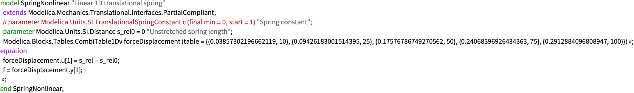
This data is provided by using the table shown in the diagram view below, which contains the data characterizing the nonlinear force-displacement relationship specific to a vulcanized hyperelastic rubber beam.
nonlinearSpring["Diagram"]modelNonlinear["SystemVariables"]What remains to be done is to assign the nonlinear spring data to the system model. The data will be assigned the variable "SpringNonlinear.nonlinearSpring.forceDisplacement".
CreateDataSystemModel["SpringNonlinear.nonlinearSpring.forceDisplacement", data]tEnd = 5;
sim = SystemModelSimulate[modelNonlinear, tEnd, <|"InitialValues" -> {"mass.m" -> mass, "mass.s" -> initialDisplacement}|>];{delta, force} = sim[{"nonlinearSpring.flange_b.s", "nonlinearSpring.flange_b.f"}, t];ParametricPlot[{delta, force}, Evaluate@Prepend[sim["SimulationInterval"], t], AspectRatio -> Full]There are two main things to keep in mind. First, you will see negative forces and movements in the results, but these did not come from the original model of the rubber beam. This happens because the modeling tool, the System Modeler, fills in these negative values by itself, using the closest positive values it has from the model. Second, you will notice that when the beam moves more (positive displacement), the force needed to move it also goes up. This means the beam gets harder to bend the more it is stretched.
nonlinearSpringDisplacementPlot = SystemModelPlot[sim, {"mass.s"}, 2, PlotStyle -> Red]nonlinearSpringForcePlot = SystemModelPlot[sim, {"nonlinearSpring.flange_b.f"}, 2, PlotStyle -> Red]Compare the hyperelastic spring to the linear elastic model of the spring.
Show[linearSpringDisplacementPlot, nonlinearSpringDisplacementPlot]Show[linearSpringForcePlot, nonlinearSpringForcePlot, PlotRange -> All]Given that the nonlinear model, represented in red, is more rigid compared to the linear model, its eigenfrequencies are higher than those of the linear model. Consequently, the displacement period in the nonlinear model is shorter than in the linear model. Additionally, the nonlinear model can withstand greater forces than the linear spring at the same level of displacement, as illustrated above.
This example demonstrates how the complexity of nonlinear PDE dynamics can be effectively simplified and captured in system-level modeling through the combined use of System Modeler and Mathematica.