

BlackmanWindow
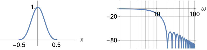
x のBlackman窓関数を表す.
詳細
- BlackmanWindowは,一般に,有限インパルス応答(FIR)フィルタ設計とスペクトル分析で使われる窓関数である.
- 窓関数は,データが短いセグメントで処理されるアプリケーションに使われ,データ値を漸減して各セグメントの終りで0に近付ける平滑化効果がある.
- Blackman窓はExactBlackmanWindowの近似である.切取り係数の結果として高周波数ロールオフが改善されるが,スペクトルのサイドローブは大きくなる.
- BlackmanWindow[x]は
に等しい. - BlackmanWindowは自動的にリストに縫い込まれる.
例題
すべて開く すべて閉じる例 (3)
スコープ (4)
BlackmanWindow[0.1]Plot[BlackmanWindow[(x - 1) / 2], {x, -1, 3}]Plot3D[BlackmanWindow[Sqrt[x ^ 2 + y ^ 2]], {x, -1, 1}, {y, -1, 1}, PlotRange -> All]ListPlot[Array[BlackmanWindow, 15, {-1 / 2, 1 / 2}], Filling -> Axis]ListPointPlot3D[Array[BlackmanWindow[#1] BlackmanWindow[#2]&, {15, 10}, {{-1 / 2, 1 / 2}}], Filling -> Axis]アプリケーション (4)
カットオフ周波数
,長さ21のローパス有限インパルス応答フィルタを作る:
h = LeastSquaresFilterKernel[{"Lowpass", π / 5}, 21]Blackman窓を使ってフィルタを漸減させることでストップバンド減衰を向上させる:
w = Array[BlackmanWindow, Length[h], {-1 / 2, 1 / 2}];
fir = h w;fir / Total[fir]Plot[Evaluate[20Log10[Abs@ListFourierSequenceTransform[#, ω]]& /@ {h, %}], {ω, 0, π}, GridLines -> Automatic]Blackman窓メソッドを使ってホワイトノイズ信号にフィルタをかける:
a = AudioGenerator["White", 1, SampleRate -> 8000];
Periodogram[{a, LowpassFilter[a, 8000 π / 3, 21, BlackmanWindow]}]窓指定を使ってサンプルPowerSpectralDensityを計算する:
proc = ARMAProcess[1, {.5}, {.3}, 1];
data = RandomFunction[proc, {50}];spec = PowerSpectralDensity[data, w, BlackmanWindow];sd = PowerSpectralDensity[data, w];sd === specプロットは,窓がスペクトル密度を平坦化したことを示している:
Plot[{sd, spec}, {w, -π, π}, PlotRange -> All, PlotLegends -> {"no window", "with window"}]Plot[{spec, Evaluate@PowerSpectralDensity[proc, w]}, {w, -π, π}, PlotLegends -> {"data", "process"}]data = RandomFunction[ARMAProcess[1, {.3}, {.4}, 1], {300}];EstimatedProcess[data, ARMAProcess[1, 1], ProcessEstimator -> {"SpectralEstimator", "Window" -> BlackmanWindow}]特性と関係 (5)
area = Integrate[BlackmanWindow[x], {x, -∞, ∞}]Plot[{BlackmanWindow[x], BlackmanWindow[x] / area}, {x, -1, 1}, PlotRange -> All]f = FourierTransform[BlackmanWindow[x], x, w]LogLinearPlot[20 Log[10, Abs[f]], {w, .1, 100}, PlotRange -> {0, -120}]Array[BlackmanWindow, 15, {-0.5, 0.5}]% / Total[%]正規化された長さ15の離散Blackman窓の離散時間フーリエ変換:
(win = Array[HammingWindow, 15, {-0.5, 0.5}];
f = ListFourierSequenceTransform[win / Total[win], ω])Plot[Abs@f, {ω, 0, π}, PlotRange -> All]tab = Table[(h = Array[win, 15, {-0.5, 0.5}];
20Log10[Abs@ListFourierSequenceTransform[h / Total[h], ω]]), {win, {BlackmanWindow, DirichletWindow}}];Plot[tab, {ω, 0, π}, PlotRange -> {5, -80}, PlotLegends -> {BlackmanWindow, DirichletWindow}]関連するガイド
テキスト
Wolfram Research (2012), BlackmanWindow, Wolfram言語関数, https://reference.wolfram.com/language/ref/BlackmanWindow.html.
CMS
Wolfram Language. 2012. "BlackmanWindow." Wolfram Language & System Documentation Center. Wolfram Research. https://reference.wolfram.com/language/ref/BlackmanWindow.html.
APA
Wolfram Language. (2012). BlackmanWindow. Wolfram Language & System Documentation Center. Retrieved from https://reference.wolfram.com/language/ref/BlackmanWindow.html
BibTeX
@misc{reference.wolfram_2026_blackmanwindow, author="Wolfram Research", title="{BlackmanWindow}", year="2012", howpublished="\url{https://reference.wolfram.com/language/ref/BlackmanWindow.html}", note=[Accessed: 13-August-2026]}
BibLaTeX
@online{reference.wolfram_2026_blackmanwindow, organization={Wolfram Research}, title={BlackmanWindow}, year={2012}, url={https://reference.wolfram.com/language/ref/BlackmanWindow.html}, note=[Accessed: 13-August-2026]}