DiscreteLQEstimatorGains[ssm,{w,v},τ]
過程のノイズと測定ノイズの共分散行列が w と v の連続時間StateSpaceModel ssm についてのサンプリング周期 τ の最適離散時間推定器ゲイン行列を与える.
DiscreteLQEstimatorGains[{ssm,sensors},{w,v},τ]
sensors を ssm のノイズの多い測定値として指定する.
DiscreteLQEstimatorGains[{ssm,sensors,dinputs},{w,v},τ]
dinputs を ssm の決定論的入力として指定する.
DiscreteLQEstimatorGains
DiscreteLQEstimatorGains[ssm,{w,v},τ]
過程のノイズと測定ノイズの共分散行列が w と v の連続時間StateSpaceModel ssm についてのサンプリング周期 τ の最適離散時間推定器ゲイン行列を与える.
DiscreteLQEstimatorGains[{ssm,sensors},{w,v},τ]
sensors を ssm のノイズの多い測定値として指定する.
DiscreteLQEstimatorGains[{ssm,sensors,dinputs},{w,v},τ]
dinputs を ssm の決定論的入力として指定する.
詳細とオプション
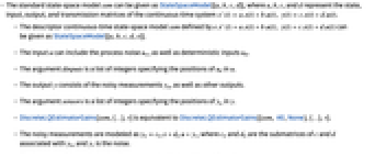
- 標準状態空間モデル ssm はStateSpaceModel[{a,b,c,d}]で与えられる.a,b,c,d は,連続時間系

の,状態,入力,出力,伝送行列を表す.
で定義されるディスクリプタ連続時間状態空間モデル ssm はStateSpaceModel[{a,b,c,d,e}]で与えられる.- 入力
は過程のノイズ
と決定論的入力
を含むことができる. - 引数 dinputs は
における
の位置を指定する整数のリストである. - 出力
はノイズの多い測定値
と他の出力からなる. - 引数 sensors は
における
の位置を指定する整数のリストである. - DiscreteLQEstimatorGains[ssm,{…},τ]はDiscreteLQEstimatorGains[{ssm, All,None},{…},τ]に等しい.
- ノイズの多い測定は

でモデル化できる.
と
は
と関連する
と
の部分行列であり,
はノイズである. - 過程のノイズと測定ノイズはホワイトノイズとガウスのノイズであると想定される.
-

, 
過程のノイズ
, 
測定ノイズ - 最適ゲインを持つ推定器は
を最小化する.
は推定状態ベクトルである. - DiscreteLQEstimatorGainsはノイズ行列を離散化したものに基づく推定器ゲインを計算する.
- 状態空間モデル ssm は0次ホールドメソッドで離散化される.
例題
すべて開く すべて閉じる例 (1)
スコープ (3)
ssm = StateSpaceModel[{{{-1.7, 50, 160}, {0.22, -1.4, -32}, {0, 0, -12}},
{{-272, 0.02, 0.1}, {0, -0.0035, 0.004}, {14, 0, 0}}, {{1, 0, 0}, {0, 1, 0}},
{{0, 0, 0}, {0, 0, 0}}}, SamplingPeriod -> None, SystemsModelLabels -> None];DiscreteLQEstimatorGains[ssm, {(| | | |
| ----- | ----- | ----- |
| 0.001 | 0 | 0 |
| 0 | 0.001 | 0 |
| 0 | 0 | 0.001 |), (| | |
| - | - |
| 1 | 0 |
| 0 | 1 |)}, 0.5]//MatrixFormDiscreteLQEstimatorGains[{ssm, 2}, {(| | | |
| ----- | ----- | ----- |
| 0.001 | 0 | 0 |
| 0 | 0.001 | 0 |
| 0 | 0 | 0.001 |), (1)}, 0.5]//MatrixFormssm = StateSpaceModel[{{{0, 0, 1, 0}, {0, 0, 0, 1}, {-29.4, 19.6, 0, 0}, {14.7, -14.7, 0, 0}},
{{0, 1, 0, 0, 0}, {0, 0, 1, 0, 0}, {0, 0, 0, 1, 0}, {0.125, 0, 0, 0, 1}},
{{1, 0, 0, 0}, {0, 0, 1, 0}}, {{0, 0, 0, 0, 0}, {0, 0, 0, 0, 0}}}, SamplingPeriod -> None,
SystemsModelLabels -> None];DiscreteLQEstimatorGains[{ssm, All, {1}}, {10^6(| | | | |
| - | - | - | - |
| 1 | 0 | 0 | 0 |
| 0 | 1 | 0 | 0 |
| 0 | 0 | 1 | 0 |
| 0 | 0 | 0 | 1 |), (| | |
| - | - |
| 1 | 0 |
| 0 | 1 |)}, 0.2]DiscreteLQEstimatorGains[StateSpaceModel[{{{-0.3, 0.65, 0}, {0, -1, 1}, {0.25, -0.5, -0.6}},
{{-1, 0}, {0.5, 0}, {0.7, -0.6}}, {{1, 0, 0}, {0, -1, -1}}, {{0, 0}, {0, 0}},
{{3, 0, 0}, {0, 5, 0}, {0, 0, 0}}}, SamplingPeriod -> None, SystemsModelLabels -> None], {(| | |
| -- | -- |
| 1. | 0. |
| 0 | 2. |), (| | |
| -- | -- |
| 5. | .1 |
| .1 | 3. |)}, .1]特性と関係 (1)
DiscreteLQEstimatorGainsを使って推定器ゲインを求める:
ssm = StateSpaceModel[{{{0, 1, 0}, {-1, -1, 0}, {0, 0, -1}}, {{0, 0}, {1, 0}, {0, 1}}, {{2, 1, 1}},
{{0, 0}}}, SamplingPeriod -> None, SystemsModelLabels -> None];Subscript[l, 1] = DiscreteLQEstimatorGains[{ssm, All, 1}, {(16), (1)}, 0.5]//Chopゲインと離散化されたモデルから離散時間Kalman推定器を作る:
kalman1 = StateOutputEstimator[{ToDiscreteTimeModel[ssm, 0.5, Method -> "ZeroOrderHold"], All, 1}, Subscript[l, 1]];これは連続時間推定器を離散化することで得られた推定器とは異なる:
kalman2 = ToDiscreteTimeModel[KalmanEstimator[{ssm, All, 1}, {(16), (1)}], 0.5, Method -> "ZeroOrderHold"];過程のノイズと測定ノイズが存在するときの最初の推定器の応答:
pnoise = Interpolation[Thread[{Range[0, 20], RandomReal[NormalDistribution[0, 4], {21}]}], t];mnoise = Interpolation[Thread[{Range[0, 20], RandomReal[NormalDistribution[0, 1], {21}]}], t];noisyout = OutputResponse[ssm, {UnitStep[t], pnoise}, {t, 20}] + mnoise;res1 = OutputResponse[kalman1, {UnitStep[t], noisyout[[1]]}, {t, 20}];res2 = OutputResponse[kalman2, {UnitStep[t], noisyout[[1]]}, {t, 20}];Show[{ListPlot[res1, Joined -> True], ListPlot[res2, PlotStyle -> Dashed, Joined -> True]}, PlotRange -> All]考えられる問題 (1)
DiscreteLQEstimatorGains[StateSpaceModel[{{{-1, 0, 0}, {0, 2, 0}, {0, 0, 3}}, {{1, 1}, {-1, 0}, {0, 1}},
{{1, 0, 0}, {0, 0, 1}}, {{0, 0}, {0, 0}}}, SamplingPeriod -> None, SystemsModelLabels -> None], {(| | |
| - | - |
| 1 | 0 |
| 0 | 1 |), (| | |
| - | - |
| 1 | 0 |
| 0 | 1 |)}, 0.1]関連するガイド
テキスト
Wolfram Research (2010), DiscreteLQEstimatorGains, Wolfram言語関数, https://reference.wolfram.com/language/ref/DiscreteLQEstimatorGains.html (2012年に更新).
CMS
Wolfram Language. 2010. "DiscreteLQEstimatorGains." Wolfram Language & System Documentation Center. Wolfram Research. Last Modified 2012. https://reference.wolfram.com/language/ref/DiscreteLQEstimatorGains.html.
APA
Wolfram Language. (2010). DiscreteLQEstimatorGains. Wolfram Language & System Documentation Center. Retrieved from https://reference.wolfram.com/language/ref/DiscreteLQEstimatorGains.html
BibTeX
@misc{reference.wolfram_2026_discretelqestimatorgains, author="Wolfram Research", title="{DiscreteLQEstimatorGains}", year="2012", howpublished="\url{https://reference.wolfram.com/language/ref/DiscreteLQEstimatorGains.html}", note=[Accessed: 11-September-2026]}
BibLaTeX
@online{reference.wolfram_2026_discretelqestimatorgains, organization={Wolfram Research}, title={DiscreteLQEstimatorGains}, year={2012}, url={https://reference.wolfram.com/language/ref/DiscreteLQEstimatorGains.html}, note=[Accessed: 11-September-2026]}