DiscreteLQRegulatorGains[sspec,wts,τ]
重み wts の費用関数を最小にする連続時間系指定 sspec のサンプリング周期 τ による離散時間状態フィードバックゲインを与える.
DiscreteLQRegulatorGains[…,"prop"]
特性"prop"の値を与える.
DiscreteLQRegulatorGains
DiscreteLQRegulatorGains[sspec,wts,τ]
重み wts の費用関数を最小にする連続時間系指定 sspec のサンプリング周期 τ による離散時間状態フィードバックゲインを与える.
DiscreteLQRegulatorGains[…,"prop"]
特性"prop"の値を与える.
詳細とオプション
- DiscreteLQRegulatorGainsは,離散線形二次調整器,離散線形二次調整器相当,あるいは離散線形二次エミュレーテッド調整器としても知られている.
- DiscreteLQRegulatorGainsは,一般に,調整コントローラあるいは追跡コントローラのデジタル実装の計算に使われる.
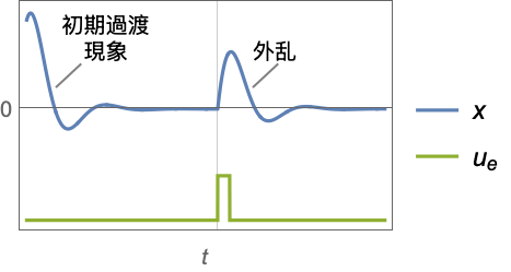
- 調整コントローラは,系を乱そうとする外乱
があっても系を平衡状態に保とうとする.典型的な例として,直立した倒立振子や水平飛行中の航空機等が挙げられる. - 調整コントローラは

の形の制御規則で与えられる.ただし,
は計算されたゲイン行列である. - 連続時間費用関数は
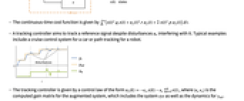
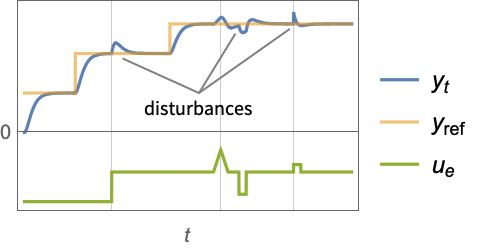
で与えられる. - 追跡コントローラは,それを妨害する外乱
があっても参照信号を追跡しようとする.典型的な例として,自動車のクルーズコントロールシステムやロボットの経路追跡が挙げられる. - 追跡コントローラは

の形の制御規則で与えられる.ただし,
は系 sys と
のダイナミクスを含む拡張系のための計算されたゲイン行列である. - 近似離散時間系:
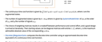
- 連続時間費用関数は

で与えられる.ただし,
は拡張状態である. - 拡張状態の数は
で与えられる.ただし,
は sys のSystemsModelOrderで,
は yref の次数で,
は信号 yrefの数で与えられる. - 重み行列の選択は,結果としてパフォーマンスと制御努力のトレードオフとなり,優れた設計に反復的に到達する.初期値は成分が
の対角行列でよい.ただし,ziは対応する xiまたは uiの許容可能な最大絶対値である. - DiscreteLQRegulatorGainsは,連続時間費用関数に相当する離散時間の近似を使って離散時間コントローラを計算する.
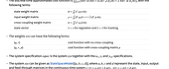
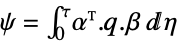
- 離散時間近似費用関数は以下の項を持つ
である. -
状態重み行列 
入力重み行列 
クロスカップリング重み行列 
状態ベクトル 調整には
,追跡には 
- 重み wts は次の形でよい.
-
{q,r} クロスカップリングがない費用関数 {q,r,p} クロスカップリング行列 p がある費用関数 - 系の指定 sspec は,系 sys と指定 uf,yt,yrefである.
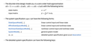
- 系 sys はStateSpaceModel[{a,b,c,d}]として与えることができる.ただし,a, b, c, d は,連続時間系

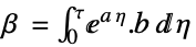
の,状態,入力,出力,フィードスルー行列である. - 離散時間設計モデル dsys は次の項を持つ0次のホールド近似

である. -
状態行列 
入力行列 
- 系の指定 sspec は以下の形でよい.
-
StateSpaceModel[…] 線形制御入力と線形状態 AffineStateSpaceModel[…] 線形制御入力と非線形状態 NonlinearStateSpaceModel[…] 非線形制御入力と非線形状態 SystemModel[…] 一般的な系のモデル <|…|> Associationとして与えられる詳細な系の指定 - 系の指定の詳細は次のキーを持つことができる.
-
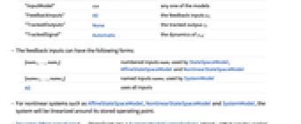
"InputModel" sys モデルの任意のもの "FeedbackInputs" All フィードバック入力 uf "TrackedOutputs" None 追跡された出力 yt "TrackedSignal" Automatic yrefのダイナミクス - フィードバック入力は次の形でよい.
-
{num1,…,numn} StateSpaceModel, AffineStateSpaceModel,NonlinearStateSpaceModelで使われる番号付き入力 numi {name1,…,namen} SystemModelで使われる名前付き入力 namei All すべての入力を使う - AffineStateSpaceModel,NonlinearStateSpaceModel,SystemModelのような非線形系については,系は保存された動作点の周りで線形化される.
- DiscreteLQRegulatorGains[…,"Data"]は cd["prop"]の形で追加的な特性の抽出に使えるSystemsModelControllerDataオブジェクト cd を返す.
- DiscreteLQRegulatorGains[…,"prop"]を使って cd["prop"]の値を直接与えることができる.
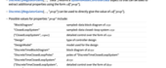
- 次は,特性"prop"の可能な値である.
-
"BlockDiagram" csys のブロック図 "ClosedLoopSystem" サンプルデータ閉ループ系 csys {"ClosedLoopSystem",cspec} csys の形式についての詳細制御 "Design" コントローラ設計のタイプ "DesignModel" 設計に使用されるモデル "DiscreteTimeBlockDiagram" dcsys のブロック図 "DiscreteTimeClosedLoopPoles" "DiscreteTimeClosedLoopSystem"の極 "DiscreteTimeClosedLoopSystem" dcsys {"DiscreteTimeClosedLoopSystem",cspec} dsys の形式に対する詳細制御 "DiscreteTimeControllerModel" dcm "DiscreteTimeDesignModel" 近似された離散時間モデル dsys "DiscreteTimeFeedbackGainsModel" dgm または {dgm1,dgm2} "DiscreteTimeOpenLoopPoles" dsys の極 "DiscreteTimeWeights" 近似された費用の重み ϕ, ρ, π "FeedbackGains" ゲイン行列 κ またはそれに相当するもの "FeedbackInputs" フィードバックに使われる sys の入力 uf "InputCount" sys の入力 u の数 "InputModel" 入力モデル sys "OpenLoopPoles" "DesignModel"の極 "OutputCount" sys の出力 y の数 "SamplingPeriod" サンプリング period τ "StateCount" sys の状態 x の数 "TrackedOutputs" 追跡された sys の出力 ytの数 - 次は, cspec の可能なキーである.
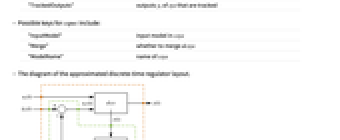
-
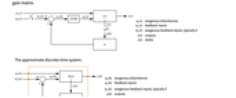
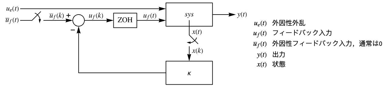
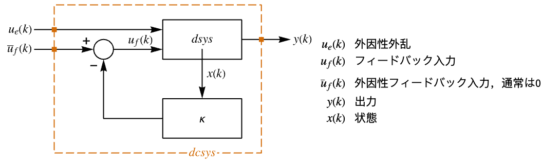
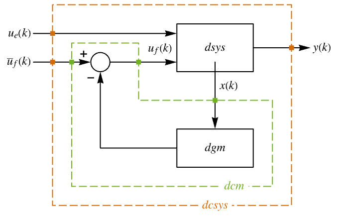
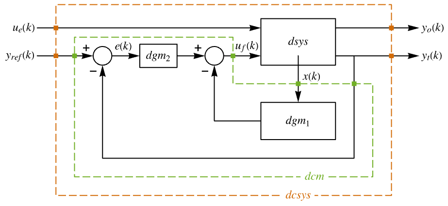
"InputModel" csys の入力モデル "Merge" csys を統合するどうか "ModelName" csys の名前 - 次は,近似離散時間調整器のレイアウトの線図である.
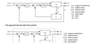
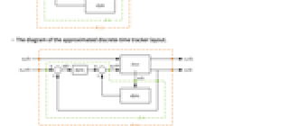
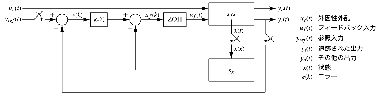
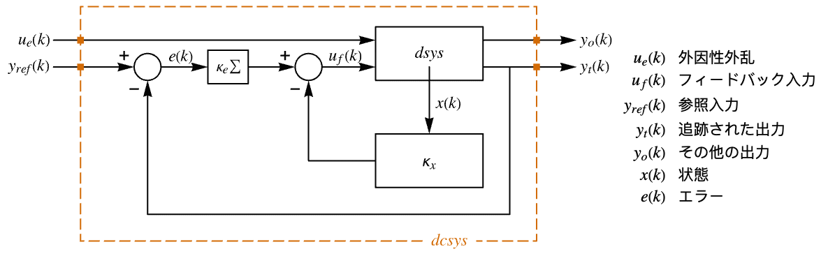
- 次は,近似離散時間追跡器のレイアウトの線図である.
例題
すべて開く すべて閉じる例 (4)
フィードバック入力 uf,外因性入力 ueである系の指定 sspec:
sspec = <|"InputModel" -> StateSpaceModel[{{{2, 1}, {4, -5}}, {{1, 0}, {0, 0.1}}, {{1, 0}}, {{0, 0}}},
SamplingPeriod -> None, SystemsModelLabels ->
{{Subscript[u, f], Subscript[u, e]}}], "FeedbackInputs" -> 1|>;wts = {(| | |
| -- | -- |
| 10 | 0 |
| 0 | 10 |), {{0.1}}};
τ = 0.5;DiscreteLQRegulatorGains[sspec, wts, τ]nssm = NonlinearStateSpaceModel[{{-1 + 3*Subscript[x, 2],
u + 2*Subscript[x, 1] - Subscript[x, 2]},
{Subscript[x, 1] + Subscript[x, 2]}},
{{Subscript[x, 1], 0}, {Subscript[x, 2], 1}}, {{u, 1}},
{Automatic}, Automatic, SamplingPeriod -> None];wts = {(| | |
| - | - |
| 1 | 0 |
| 0 | 1 |), {{0.25}}};
τ = 0.2;DiscreteLQRegulatorGains[nssm, wts, τ]sspec = <|"InputModel" -> StateSpaceModel[{{{3, 0}, {-1, 5}}, {{0, 1}, {1, 0}}, {{1, 0}}, {{0, 0}}}, SamplingPeriod -> None,
SystemsModelLabels -> None], "TrackedOutputs" -> 1|>;wts = {(| | | |
| -- | ---- | -- |
| 10 | 0 | 0 |
| 0 | 10^2 | 0 |
| 0 | 0 | 10 |), (| | |
| - | - |
| 1 | 0 |
| 0 | 1 |)};
τ = 0.1;DiscreteLQRegulatorGains[sspec, wts, τ]ssm = StateSpaceModel[{{{0., 1.}, {-6., 5.}}, {{0.}, {1.}}, {{1, 0}}, {{0.}}}, SamplingPeriod -> None,
SystemsModelLabels -> None];wts = {(| | |
| - | - |
| 1 | 0 |
| 0 | 1 |), {{0.25}}};
τ = 0.2;dlqr = DiscreteLQRegulatorGains[ssm, wts, τ, "Data"]{olPoles, clPoles} = dlqr[{"OpenLoopPoles", "DiscreteTimeClosedLoopPoles"}]PoleZeroPlot[dlqr["InputModel"]]PoleZeroPlot[dlqr["DiscreteTimeClosedLoopSystem"]]スコープ (30)
基本的な用法 (7)
ssm = StateSpaceModel[{{{-1}}, {{1}}}, SamplingPeriod -> None, SystemsModelLabels -> None];κ = DiscreteLQRegulatorGains[ssm, {{{1}}, {{1}}}, 0.1]dssm = ToDiscreteTimeModel[ssm, 0.1, Method -> "ZeroOrderHold"]SystemsModelStateFeedbackConnect[dssm, κ]ssm = StateSpaceModel[{{{-1}}, {{1}}}, SamplingPeriod -> None, SystemsModelLabels -> None];κ = DiscreteLQRegulatorGains[ssm, {{{1}}, {{1}}}, 0.1]dssm = ToDiscreteTimeModel[ssm, 0.1, Method -> "ZeroOrderHold"]SystemsModelStateFeedbackConnect[dssm, κ]ssm = StateSpaceModel[{{{-1}}, {{1}}}, SamplingPeriod -> None, SystemsModelLabels -> None];
vl = {0.01, 0.1, 1.0};κ = Table[DiscreteLQRegulatorGains[ssm, {{{1}}, {{1}}}, τ], {τ, vl}]dssm = Table[ToDiscreteTimeModel[ssm, τ, Method -> "ZeroOrderHold"], {τ, vl}]MapThread[SystemsModelStateFeedbackConnect, {dssm, κ}]ssm = StateSpaceModel[{{{-3, 0}, {0, -1}}, {{0.5}, {-0.5}}, {{-1, -1}}, {{0}}}, SamplingPeriod -> None,
SystemsModelLabels -> None];κ = DiscreteLQRegulatorGains[ssm, {(| | |
| - | - |
| 5 | 0 |
| 0 | 5 |), (1)}, 0.5]Dimensions[κ]{SystemsModelDimensions[ssm][[1]], SystemsModelOrder[ssm]}ssm = StateSpaceModel[{{{0, 0, -5}, {1, 0, -9.5}, {0, 1, -5.5}}, {{-5, 1}, {-4.5, 0}, {-1, 0}},
{{0, 0, 1}}, {{1, 0}}}, SamplingPeriod -> None, SystemsModelLabels -> None];MatrixForm[κ1 = DiscreteLQRegulatorGains[ssm, {(| | | |
| - | - | - |
| 1 | 0 | 0 |
| 0 | 1 | 0 |
| 0 | 0 | 1 |), (| | |
| - | - |
| 1 | 0 |
| 0 | 2 |)}, 0.1]]MatrixForm[κ2 = DiscreteLQRegulatorGains[ssm, {(| | | |
| - | - | - |
| 1 | 0 | 0 |
| 0 | 1 | 0 |
| 0 | 0 | 1 |), (| | |
| - | - |
| 2 | 0 |
| 0 | 1 |)}, 0.1]]Norm /@ κ1
Norm /@ κ2Norm /@ DiscreteLQRegulatorGains[ssm, {(| | | |
| - | - | - |
| 1 | 0 | 0 |
| 0 | 1 | 0 |
| 0 | 0 | 1 |), (| | |
| -- | - |
| 10 | 0 |
| 0 | 1 |)}, 0.1]費用関数が状態とフィードバック入力のクロスカップリングを含む場合のゲインを計算する:
ssm = StateSpaceModel[{{{1, 0, 0}, {0, -2, 0}, {0, 0, 3}}, {{0, 0, -1}, {1, 0, -2}, {0.1, 0, 0.5}},
{{1, 0, 0}}, {{0, 0, 0}}}, SamplingPeriod -> None, SystemsModelLabels -> None];
MatrixForm[DiscreteLQRegulatorGains[ssm, {(| | | |
| -- | --- | - |
| 10 | 0 | 0 |
| 0 | 0.1 | 0 |
| 0 | 0 | 1 |), (| | | |
| - | - | - |
| 1 | 0 | 0 |
| 0 | 1 | 0 |
| 0 | 0 | 1 |), (| | | |
| - | - | - |
| 1 | 2 | 0 |
| 2 | 0 | 0 |
| 0 | 1 | 1 |)}, 1]]nssm = NonlinearStateSpaceModel[{{x2, u*(1 + x1) +
x1*x2 + Cos[x1]}, {x1}},
{{x1, 0}, {x2, -1}}, {{u, -1}}, {Automatic}, Automatic,
SamplingPeriod -> None];DiscreteLQRegulatorGains[nssm, {(| | |
| - | - |
| 1 | 0 |
| 0 | 1 |), (1)}, 0.1]ssm = StateSpaceModel[nssm];DiscreteLQRegulatorGains[ssm, {(| | |
| - | - |
| 1 | 0 |
| 0 | 1 |), (1)}, 0.1]工場のモデル (5)
DiscreteLQRegulatorGains[StateSpaceModel[{{{0, 1, 0}, {0, 0, 1}, {5, 9, 3}}, {{0}, {0}, {1}}, {{8, 2, 1}}, {{0}}},
SamplingPeriod -> None, SystemsModelLabels -> None], {(| | | |
| - | -- | -- |
| 1 | 0 | 0 |
| 0 | 10 | 0 |
| 0 | 0 | 10 |), (1)}, 0.1]ディスクリプタStateSpaceModel:
DiscreteLQRegulatorGains[StateSpaceModel[{{{-0.3, 0.65, 0}, {0, 1, 0}, {0.25, -0.5, -0.6}}, {{-1}, {0.5}, {0.7}},
{{1, 0, 0}}, {{0}}, {{3, 0, 0}, {5, 0, 0}, {0, 1, 0}}}, SamplingPeriod -> None,
SystemsModelLabels -> None], {(| | | |
| - | - | - |
| 4 | 0 | 0 |
| 0 | 3 | 0 |
| 0 | 0 | 5 |), (1)}, .1]DiscreteLQRegulatorGains[AffineStateSpaceModel[{{Sin[Subscript[x, 1]] + Subscript[x, 2],
-Subscript[x, 1] - Subscript[x, 2]},
{{Subscript[x, 1]}, {1}}, {Subscript[x, 1]}, {{0}}},
{Subscript[x, 1], Subscript[x, 2]}, {{u, 0}}, {Automatic},
Automatic, SamplingPeriod -> None], {(| | |
| - | - |
| 1 | 0 |
| 0 | 1 |), (1)}, 0.1]DiscreteLQRegulatorGains[NonlinearStateSpaceModel[
{{Subscript[x, 2] + Subscript[x, 1]*Subscript[x, 2],
u + Subscript[x, 1]}, {Subscript[x, 1]}},
{Subscript[x, 1], Subscript[x, 2]}, {u}, {Automatic},
Automatic, SamplingPeriod -> None], {(| | |
| - | - |
| 1 | 0 |
| 0 | 1 |), (1)}, 0.1]sm = CreateSystemModel[{x''[t] + x'[t] + x[t] == u[t], y[t] == x[t]}, t, {"u"∈"Modelica.Blocks.Interfaces.RealInput", "y"∈"Modelica.Blocks.Interfaces.RealOutput"}];DiscreteLQRegulatorGains[sm, {(| | |
| - | - |
| 1 | 0 |
| 0 | 1 |), (1)}, 0.1]特性 (14)
DiscreteLQRegulatorGainsは,デフォルトで,離散時間フィードバックゲインを返す:
DiscreteLQRegulatorGains[StateSpaceModel[{{{0, 1}, {-1, -2}}, {{0}, {1}}, {{1, 0}}, {{0}}}, SamplingPeriod -> None,
SystemsModelLabels -> None], {(| | |
| - | - |
| 1 | 0 |
| 0 | 1 |), (1)}, 1.0]% == DiscreteLQRegulatorGains[StateSpaceModel[{{{0, 1}, {-1, -2}}, {{0}, {1}}, {{1, 0}}, {{0}}}, SamplingPeriod -> None,
SystemsModelLabels -> None], {(| | |
| - | - |
| 1 | 0 |
| 0 | 1 |), (1)}, 1.0, "FeedbackGains"]κ = DiscreteLQRegulatorGains[NonlinearStateSpaceModel[
{{-Subscript[x, 1] + u*Subscript[x, 1] +
Subscript[x, 2]/E^Subscript[x, 1],
E^Subscript[x, 2] - Subscript[x, 1]}, {Subscript[x, 2]}},
{{Subscript[x, 1], 1}, {Subscript[x, 2], 0}}, {{u, 1.}},
{Automatic}, Automatic, SamplingPeriod -> None], {(| | |
| - | - |
| 1 | 0 |
| 0 | 1 |), (1)}, 1.0]κ0+κ1.x の形式をしている.ただし,κ0と κ1は定数である:
{κ0, κ1} = {κ /. {Subscript[x, _] -> 0}, D[κ, {{Subscript[x, 1], Subscript[x, 2]}}]}DiscreteLQRegulatorGains[StateSpaceModel[{{{0, 1}, {-1, -2}}, {{0}, {1}}, {{1, 0}}, {{0}}}, SamplingPeriod -> None,
SystemsModelLabels -> None], {(| | |
| - | - |
| 1 | 0 |
| 0 | 1 |), (1)}, 1.0, "DiscreteTimeFeedbackGainsModel"]DiscreteLQRegulatorGains[NonlinearStateSpaceModel[{{Subscript[x, 2], -2/3 + u -
Subscript[x, 1]/3 - Subscript[x, 2]/2},
{Subscript[x, 1]}}, {{Subscript[x, 1], 1},
{Subscript[x, 2], 0}}, {{u, 1.}}, {Automatic}, Automatic,
SamplingPeriod -> None], {(| | |
| - | - |
| 1 | 0 |
| 0 | 1 |), (1)}, 1.0, "DiscreteTimeFeedbackGainsModel"]DiscreteLQRegulatorGains[StateSpaceModel[{{{0., 1.}, {-0.05, -0.9}}, {{0}, {1}}, {{1, 0}}, {{0}}},
{Subscript[x, 1], Subscript[x, 2]}, {{f, 0}},
SamplingPeriod -> None, SystemsModelLabels -> None], {(| | |
| - | - |
| 1 | 0 |
| 0 | 1 |), (1)}, 1.0, "DiscreteTimeClosedLoopSystem"]DiscreteLQRegulatorGains[StateSpaceModel[{{{0., 1.}, {-0.05, -0.9}}, {{0}, {1}}, {{1, 0}}, {{0}}},
{Subscript[x, 1], Subscript[x, 2]}, {{f, 0}},
SamplingPeriod -> None, SystemsModelLabels -> None], {(| | |
| - | - |
| 1 | 0 |
| 0 | 1 |), (1)}, 1.0, "DiscreteTimeBlockDiagram"]DiscreteLQRegulatorGains[StateSpaceModel[{{{0., 1.}, {-0.05, -0.9}}, {{0}, {1}}, {{1, 0}}, {{0}}},
{Subscript[x, 1], Subscript[x, 2]}, {{f, 0}},
SamplingPeriod -> None, SystemsModelLabels -> None], {(| | |
| - | - |
| 1 | 0 |
| 0 | 1 |), (1)}, 1.0, "ClosedLoopSystem"]DiscreteLQRegulatorGains[StateSpaceModel[{{{0., 1.}, {-0.05, -0.9}}, {{0}, {1}}, {{1, 0}}, {{0}}},
{Subscript[x, 1], Subscript[x, 2]}, {{f, 0}},
SamplingPeriod -> None, SystemsModelLabels -> None], {(| | |
| - | - |
| 1 | 0 |
| 0 | 1 |), (1)}, 1.0, "BlockDiagram"]assm = AffineStateSpaceModel[{{Subscript[x, 2], -0.05*Subscript[x, 1] -
0.9*Subscript[x, 2]^2}, {{0}, {1}}, {Subscript[x, 1]}, {{0}}},
{Subscript[x, 1], Subscript[x, 2]}, {{f, 0}}, {Automatic},
Automatic, SamplingPeriod -> None];
{wts, τ} = {{(| | |
| - | - |
| 1 | 0 |
| 0 | 1 |), (1)}, 1.0};DiscreteLQRegulatorGains[assm, wts, τ, "DiscreteTimeClosedLoopPoles"]DiscreteLQRegulatorGains[assm, {10wts[[1]], wts[[2]]}, τ, "DiscreteTimeClosedLoopPoles"]DiscreteLQRegulatorGains[assm, {wts[[1]], 10wts[[2]]}, τ, "DiscreteTimeClosedLoopPoles"]assm = AffineStateSpaceModel[{{Subscript[x, 2], -0.05*Subscript[x, 1] -
0.9*Subscript[x, 2]^2}, {{0}, {1}}, {Subscript[x, 1]}, {{0}}},
{Subscript[x, 1], Subscript[x, 2]}, {{f, 0}}, {Automatic},
Automatic, SamplingPeriod -> None];
{wts, τ} = {{(| | |
| - | - |
| 1 | 0 |
| 0 | 1 |), (1)}, 1.0};DiscreteLQRegulatorGains[assm, wts, τ, "DesignModel"]DiscreteLQRegulatorGains[assm, wts, τ, "OpenLoopPoles"]DiscreteLQRegulatorGains[assm, wts, τ, "DiscreteTimeDesignModel"]DiscreteLQRegulatorGains[assm, wts, τ, "DiscreteTimeOpenLoopPoles"]DiscreteLQRegulatorGains[AffineStateSpaceModel[{{Subscript[x, 2], -0.05*Subscript[x, 1] -
0.9*Subscript[x, 2]^2}, {{0}, {1}}, {Subscript[x, 1]}, {{0}}},
{Subscript[x, 1], Subscript[x, 2]}, {{f, 0}}, {Automatic},
Automatic, SamplingPeriod -> None], {(| | |
| - | - |
| 1 | 0 |
| 0 | 1 |), (1)}, 1.0, "DiscreteTimeWeights"];MatrixForm /@ %DiscreteLQRegulatorGains[AffineStateSpaceModel[{{Subscript[x, 2], -0.05*Subscript[x, 1] -
0.9*Subscript[x, 2]^2}, {{0}, {1}}, {Subscript[x, 1]}, {{0}}},
{Subscript[x, 1], Subscript[x, 2]}, {{f, 0}}, {Automatic},
Automatic, SamplingPeriod -> None], {(| | |
| - | - |
| 1 | 0 |
| 0 | 1 |), (1)}, 1.0, "Design"]Dataset[Table[{prop, DiscreteLQRegulatorGains[IconizedObject[«sys»], IconizedObject[«wts»], 1.0, prop]}, {prop, IconizedObject[«props»]}]]𝒸𝒹 = DiscreteLQRegulatorGains[IconizedObject[«sspec»], IconizedObject[«wts»], 1.0, "Data"]𝒸𝒹["Properties"]𝒸𝒹["DiscreteTimeClosedLoopPoles"]追跡 (4)
sspec = <|"InputModel" -> StateSpaceModel[{{{0, 7}, {-1, -6}}, {{0}, {1}}, {{5, 0}}, {{0}}}, SamplingPeriod -> None,
SystemsModelLabels -> None], "TrackedOutputs" -> 1|>;𝒸𝒹 = DiscreteLQRegulatorGains[sspec, {(| | | |
| --- | - | --- |
| 100 | 0 | 0 |
| 0 | 1 | 0 |
| 0 | 0 | 0.5 |), (1)}, 0.75, "Data"]OutputResponse[𝒸𝒹["DiscreteTimeClosedLoopSystem"], ref = Table[1, 30]];
ListStepPlot[{ref, %[[1]]}, IconizedObject[«plotOpts»]]𝒸𝒹["DiscreteTimeBlockDiagram"]sspec = <|"InputModel" -> StateSpaceModel[{{{2., 0}, {0, -2}}, {{1., 0}, {0, 1}}, {{1, 0}, {3., 1}}, {{0, 0}, {0, 0}}},
SamplingPeriod -> None, SystemsModelLabels -> None], "TrackedOutputs" -> {1, 2}|>;𝒸𝒹 = DiscreteLQRegulatorGains[sspec, {(| | | | |
| - | - | --- | --- |
| 1 | 0 | 0 | 0 |
| 0 | 1 | 0 | 0 |
| 0 | 0 | 100 | 0 |
| 0 | 0 | 0 | 100 |), (| | |
| - | - |
| 1 | 0 |
| 0 | 1 |)}, 0.75, "Data"]refs = Table[ConstantArray[RandomInteger[{-12, -4}], 30], 2];
or = OutputResponse[𝒸𝒹["DiscreteTimeClosedLoopSystem"], refs];ListStepPlot[Riffle[refs, or], IconizedObject[«plotOpts»]]sspec = <|"InputModel" -> StateSpaceModel[{{{0, 1}, {-5, -3}}, {{0}, {1}}, {{5, 0}}, {{0}}}, SamplingPeriod -> None,
SystemsModelLabels -> None], "TrackedOutputs" -> 1|>;𝒸𝒹 = DiscreteLQRegulatorGains[sspec, {(| | | |
| -- | - | -- |
| 10 | 0 | 0 |
| 0 | 1 | 0 |
| 0 | 0 | 10 |), {{1}}}, 1.0, "Data"]cm = 𝒸𝒹["DiscreteTimeControllerModel"]ref = Table[1, 30]dcsys = 𝒸𝒹["DiscreteTimeClosedLoopSystem"];Short[sr = StateResponse[dcsys, {ref}]]Short[or = OutputResponse[dcsys, {ref}]]cinps = Join[{ref}, or, sr];OutputResponse[cm, cinps];
ListStepPlot[%[[1]], PlotRange -> All]tSig = Function[{r, t}, r''[t] + 0.5r[t]]m = Max[Join[Cases[tSig[r, t], Derivative[n_][r][t] :> n], {0}]]ref = DSolveValue[{tSig[r, t] == 0, r[0] == 0, r'[0] == 1}, r[t], t]
dref = Table[ref, {t, 0, 20 π, τ = 0.4}];
len = Length[dref]ListStepPlot[dref, DataRange -> {0, τ (len - 1)}]sspec = <|"InputModel" -> StateSpaceModel[{{{-1}}, {{1}}, {{1}}, {{0}}}, SamplingPeriod -> None, SystemsModelLabels -> None], "TrackedOutputs" -> 1, "TrackedSignal" -> tSig|>;{q, k} = {Length[sspec["TrackedOutputs"]], SystemsModelOrder[sspec["InputModel"]]}{qq, rr} = {(| | | |
| - | --- | - |
| 1 | 0 | 0 |
| 0 | 100 | 0 |
| 0 | 0 | 1 |), {{0.01}}};
Join[Dimensions[qq], {k + m q}]𝒸𝒹 = DiscreteLQRegulatorGains[sspec, {qq, rr}, τ, "Data"]or = OutputResponse[𝒸𝒹["DiscreteTimeClosedLoopSystem"], dref][[1]];ListStepPlot[{dref, or}, PlotRange -> All, PlotStyle -> {Dashing[{Small, Small}], Automatic}, PlotLegends -> {"ref.", "actual"}, DataRange -> {0, τ (len - 1)}]アプリケーション (12)
機械系 (5)
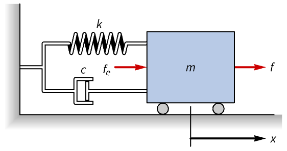
nssm = NonlinearStateSpaceModel[IconizedObject[«eqns»] /. IconizedObject[«pars»], {x[t], v[t]}, {f[t], Subscript[f, e][t]}, {x[t], v[t]}, t]外乱力 feに応答する台車の開ループ応答は調整されておらず,安定するまでに40秒ほどかかる:
OutputResponse[nssm, {0, 0.1 UnitStep[t]}, {t, 0, 60}];
Plot[%, {t, 0, 60}, PlotLegends -> {x, v}, PlotRange -> All]sspec = <|"InputModel" -> nssm, "FeedbackInputs" -> 1|>;コントローラ設計の制御重みの集合とサンプリング時間を指定する:
wts = {DiagonalMatrix[{10, 1}], {{0.1}}};
τ = 0.4;dlqr = DiscreteLQRegulatorGains[sspec, wts, τ, "Data"]dcsys = dlqr["DiscreteTimeClosedLoopSystem"]or = OutputResponse[{dcsys, {0, 0.1}}, Table[{0, 0}, 20]];
ListStepPlot[%, DataRange -> {0, 19 τ}, PlotRange -> All, PlotLegends -> {x, v}]cm = dlqr["DiscreteTimeControllerModel"]OutputResponse[cm, Join[Table[{0}, 20], or]];
ListStepPlot[%, DataRange -> {0, 19 τ}, PlotRange -> All]
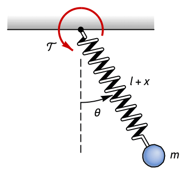
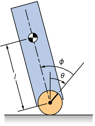
pend = NonlinearStateSpaceModel[IconizedObject[«eqns»] /. IconizedObject[«pars»], {x[t], x'[t], θ[t], θ'[t]}, 𝒯[t], {x[t], θ[t]}, t]OutputResponse[{pend, {0.1, 0, 0.2, 0}}, {0, 0}, {t, 0, 10}];
Plot[%, {t, 0, 10}, PlotRange -> All, PlotLegends -> {x, θ}]sspec = <|"InputModel" -> pend, "MeasuredOutputs" -> 2|>;コントローラ設計のための制御重みの集合とサンプリング時間を指定する:
wts = {DiagonalMatrix[{1, 1, 1, 1}], {{1}}};
τ = 0.5;dlqr = DiscreteLQRegulatorGains[sspec, wts, τ, "Data"]dcsys = dlqr["DiscreteTimeClosedLoopSystem"]sr = StateResponse[{dcsys, {0.1, 0, 0.2, 0}}, Table[{0, 0}, 60]];
ListStepPlot[{%[[1]], %[[3]]}, DataRange -> {0, 59 τ}, IconizedObject[«plotOpts»]]ControllableModelQ[StateSpaceModel[pend]]cm = dlqr["DiscreteTimeControllerModel"]OutputResponse[cm, Join[Table[{0, 0}, 60], sr]];
ListStepPlot[%, DataRange -> {0, 59 τ}, PlotRange -> All]Grid[{Table[PoleZeroPlot[{sys}, ImageSize -> Small], {sys, {dlqr["DiscreteTimeDesignModel"], dcsys}}]}, Spacings -> 2]
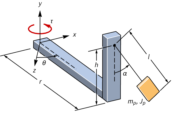
pend = NonlinearStateSpaceModel[IconizedObject[«eqns»] /. IconizedObject[«pars»], {θ[t], α[t], θ'[t], α'[t]}, Subscript[v, m][t], {θ[t], α[t]}, t]//Chop//FullSimplifyOutputResponse[{pend, {0.3, 0.2}}, 0, {t, 0, 300}];
Plot[%, {t, 0, 100}, PlotRange -> All, PlotLegends -> {θ, α}]wts = {DiagonalMatrix[{10^2, 10^4, 10, 10}], {{1}}};
τ = 0.1;dlqr = DiscreteLQRegulatorGains[pend, wts, τ, "Data"]dcsys = dlqr["DiscreteTimeClosedLoopSystem"]sr = StateResponse[{dcsys, {0.3, 0.2}}, Table[0, 150 ]];
ListStepPlot[%[[{1, 2}]], DataRange -> {0, 149 τ}, IconizedObject[«plotOpts»]]dcm = dlqr["DiscreteTimeControllerModel"]OutputResponse[dcm, Join[{Table[0, 150 ]}, sr]];
ListStepPlot[%, DataRange -> {0, 149 τ}, PlotRange -> All]
bbot = NonlinearStateSpaceModel[IconizedObject[«eqns»] /. IconizedObject[«pars»], {θ[t], ϕ[t], θ'[t], ϕ'[t]}, {Subscript[𝒯, 1][t], Subscript[𝒯, 2][t]}, {θ[t], ϕ[t]}, t]//Chop//Simplifyor = OutputResponse[{bbot, {0, 0.15, 0, 0}}, {0, 0}, {t, 0, 10}];Table[Plot[ℴ𝓇[[1]], {t, 0, 10}, IconizedObject[«plotOpts»]], {ℴ𝓇, ({or, {θ, ϕ}})}]wts = {10(| | | | |
| - | - | - | - |
| 5 | 0 | 0 | 0 |
| 0 | 5 | 0 | 0 |
| 0 | 0 | 1 | 0 |
| 0 | 0 | 0 | 1 |), 0.1(| | |
| - | - |
| 1 | 0 |
| 0 | 1 |)};
τ = 0.1;dlqr = DiscreteLQRegulatorGains[bbot, wts, τ, "Data"]dcsys = dlqr["DiscreteTimeClosedLoopSystem"]//Simplifysr = StateResponse[{dcsys, {0, 0.15, 0, 0}}, Table[{0, 0}, 60]];
ListStepPlot[{%[[1]], %[[2]]}, DataRange -> {0, 59 τ}, IconizedObject[«plotOpts»]]cm = dlqr["DiscreteTimeControllerModel"]//SimplifyOutputResponse[cm, Join[Table[{0, 0}, 60], sr]];
ListStepPlot[%, DataRange -> {0, 59 τ}, IconizedObject[«plotOpts»]]
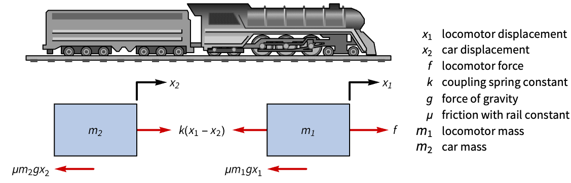
train = StateSpaceModel[IconizedObject[«eqns»] /. IconizedObject[«pars»], {Subscript[x, 1][t], Subscript[x, 2][t], Subscript[x, 1]'[t], Subscript[x, 2]'[t]}, f[t], {Subscript[x, 1][t], Subscript[x, 2][t]}, t, IconizedObject[«labels»]]機関車の位置
が変位すると,調整されていない振動が発生する:
OutputResponse[{train, {0.1, 0, 0, 0}}, 0, {t, 0, 100}];
Plot[%, {t, 0, 30}, PlotRange -> All, PlotLegends -> {Subscript[x, 1], Subscript[x, 2]}]Eigenvalues[First@Normal@train]//ChoptSig = Table[Splice[ConstantArray[i, 40]], {i, {2, 5, 9}}];
tSigPlot = ListStepPlot[%, IconizedObject[«plotOpts»]]sspec = <|"InputModel" -> train, "TrackedOutputs" -> 1|>;wts = {DiagonalMatrix[{1, 1, 1, 1, 1}], {{0.1}}};
τ = 0.2;dlqr = DiscreteLQRegulatorGains[sspec, wts, τ, "Data"]dcsys = dlqr["DiscreteTimeClosedLoopSystem"]sr = StateResponse[dcsys, tSig];Show[tSigPlot, ListStepPlot[Take[sr, 2], PlotLegends -> {Subscript[x, 1], Subscript[x, 2]}]]ListStepPlot[sr[[{3, 4}]], PlotLegends -> {Derivative[1][Subscript[x, 1]], Derivative[1][Subscript[x, 2]]}]dcm = dlqr["DiscreteTimeControllerModel"]cinps = Join[{tSig}, sr[[1 ;; 1]], sr[[1 ;; 4]]];ListStepPlot[OutputResponse[dcm, cinps]]航空宇宙系 (3)
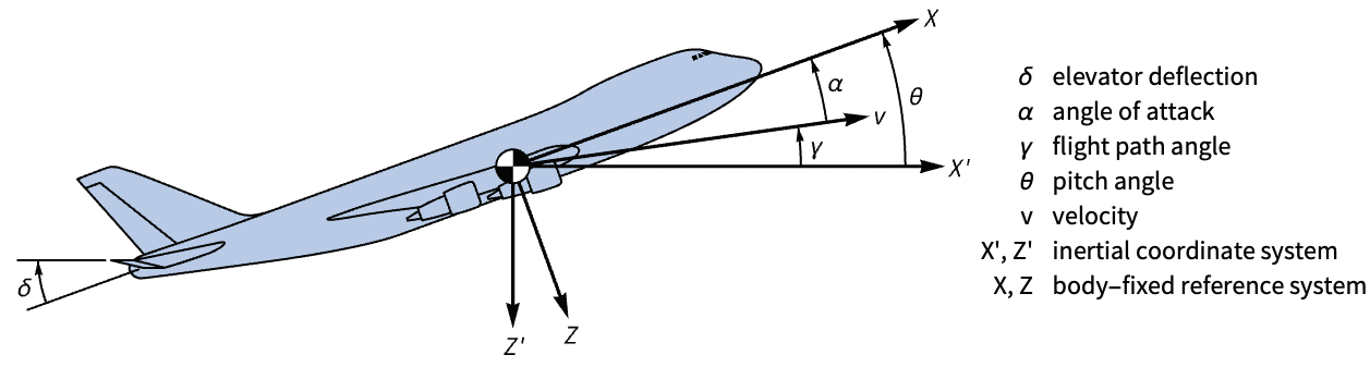
ssm = StateSpaceModel[IconizedObject[«eqns»], IconizedObject[«states»], δ[t], θ[t], t, IconizedObject[«labels»]]OutputResponse[{ssm, {0, 0, 0}}, UnitStep[t], {t, 0, 10}];
Plot[%, {t, 0, 10}, PlotRange -> All]PoleZeroPlot[ssm]離散時間LQR制御器の設計のために制御重みの集合とサンプリング時間を指定する:
wts = {DiagonalMatrix[{10, 10, 100}], {{0.1}}};
τ = 0.5;dlqr = DiscreteLQRegulatorGains[ssm, wts, τ, "Data"]dcsys = dlqr["DiscreteTimeClosedLoopSystem"]PoleZeroPlot[dcsys]sr = StateResponse[dcsys, Table[1, 30]];
ListStepPlot[sr[[3]], DataRange -> {0, 29 τ}, IconizedObject[«plotOpts»]]cm = dlqr["DiscreteTimeControllerModel"]OutputResponse[cm, Join[{Table[1, 30]}, sr]];
ListStepPlot[%, DataRange -> {0, 29 τ}, IconizedObject[«plotOpts»]]
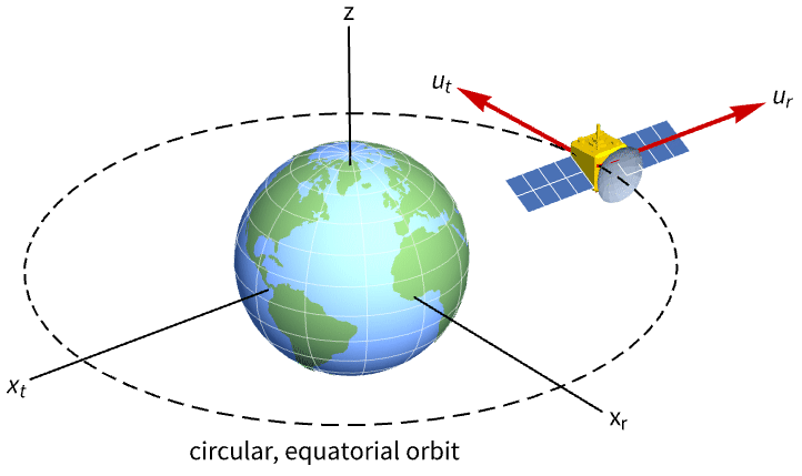
sat = StateSpaceModel[IconizedObject[«abc»], IconizedObject[«labels»]] /. ω -> 0.0011補正スラスタ入力がないと,状態の摂動によって衛星の軌道が逸れる:
OutputResponse[{sat, {0, -1, 0, 1}}, {0, 0}, {t, 0, 10800}];
Plot[%, {t, 0, 10800}, PlotRange -> All, PlotLegends -> {Subscript[x, r], Subscript[x, t]}]接線スラスタが故障した場合は軌道が制御できるが,ラジアルスラスタが故障した場合は制御できない:
Table[ControllableModelQ[SystemsModelExtract[sat, i]], {i, 2}]接線のスラスタだけを使って衛星を制御するように系の設定を行う:
sspec = <|"InputModel" -> sat, "FeedbackInputs" -> 2|>;wts = {DiagonalMatrix[{1, 100, 1, 1}], {{1}}};
τ = 0.5;dlqr = DiscreteLQRegulatorGains[sspec, wts, τ, "Data"]dcsys = dlqr["DiscreteTimeClosedLoopSystem"]sr = StateResponse[{dcsys, {0, -1, 0, 1}}, Table[{0, 0}, 5400]];
ListStepPlot[sr[[{1, 3}]], DataRange -> {0, 5399 τ}, IconizedObject[«plotOpts»]]cm = dlqr["DiscreteTimeControllerModel"]OutputResponse[cm, Join[{Table[0, 5400]}, sr]];
ListStepPlot[%, DataRange -> {0, 5399 τ}, IconizedObject[«plotOpts»]]
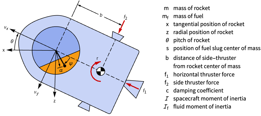
流体スロッシングを揺れる紳士として近似するロケットのモデル:
assm = AffineStateSpaceModel[IconizedObject[«eqns»] /. IconizedObject[«pars»], IconizedObject[«states»], {𝓇[t], Subscript[𝒻, 1][t], Subscript[𝒻, 2][t]}, {θ[t], ψ[t], ω[t], γ[t]}, t]OutputResponse[{assm, {0, 0.25, 0, 0, 0, -1}}, {0, 0, 0}, {t, 0, 60}];
GraphicsRow@Table[Plot[%[[i]], {t, 0, 60}, IconizedObject[«plotOpts»]], {i, 2}]8状態のうち6状態だけが制御可能なので,制御可能性行列は最大階数ではない:
ssm = StateSpaceModel[assm];
cm = ControllabilityMatrix[ssm];{MatrixRank[cm], SystemsModelOrder[ssm]}notC = Cases[Subsets[Range[8], {2}], _ ? (ControllableModelQ[SystemsModelDelete[ssm, None, None, #]]&)]Grid[Table[Part[IconizedObject[«states»], i], {i, notC}], Frame -> {True, {True, True, True}}]制御できない状態の3番目のペアを削除することで制御可能なモデルを入手する:
assmDesign = SystemsModelDelete[assm, None, None, notC[[3]]]wts = {DiagonalMatrix[{10^7, 10^6, 1, 10^5, 10^5, 10^4}], DiagonalMatrix[{0.75, 1, 0.5}]};
τ = 0.01;dlqr = DiscreteLQRegulatorGains[assmDesign, wts, τ, "Data"]dcsys = dlqr[{"DiscreteTimeClosedLoopSystem"}]//Simplify//Chop[#, 10^-5]&sr = StateResponse[{dcsys, {0, 0.25, 0, 0, -1, 0}}, Table[{0, 0, 0}, 2000]];
Table[ListStepPlot[%[[i]], DataRange -> {0, 1999 τ}, IconizedObject[«plotOpts»]], {i, 2}]dcm = dlqr["DiscreteTimeControllerModel"]OutputResponse[dcm, Join[Table[{0, 0, 0}, 2000], sr]];
ListStepPlot[%, DataRange -> {0, 1999 τ}, IconizedObject[«plotOpts»]]生物学系 (1)
nssm = NonlinearStateSpaceModel[IconizedObject[«eqns»], {Subscript[c, b][t], Subscript[c, l][t]}, {Subscript[q, gi][t], Subscript[q, iv][t]}, Subscript[c, b][t], t] /. IconizedObject[«pars»]StateSpaceModelを使って系を線形化する:
ssm = N@StateSpaceModel[nssm, IconizedObject[«labels»]]介入しなければ,人体がアルコール濃度を調整するのに
ほどかかる:
StateResponse[{ssm, {12, 3}}, {0, 0}, {t, 0, 200}];
Table[Plot[𝓈𝓇[[1]], {t, 0, 200}, IconizedObject[«plotOpts»]], {𝓈𝓇, ({%, {Subscript[c, b], Subscript[c, l]}})}]wts = {DiagonalMatrix[{10000, 1}], DiagonalMatrix[{10^2, 10^4}]};
τ = 0.5;dlqr = DiscreteLQRegulatorGains[ssm, wts, τ, "Data"]dcsys = dlqr["DiscreteTimeClosedLoopSystem"]//Simplifysr = StateResponse[{dcsys, {12, 3}}, ConstantArray[{0, 0}, 300]];
Table[ListStepPlot[𝓈𝓇[[1]], IconizedObject[«plotOpts»]], {𝓈𝓇, ({%, {Subscript[c, b], Subscript[c, l]}})}]cm = dlqr["DiscreteTimeControllerModel"]OutputResponse[cm, Join[Table[{0, 0}, 300], sr]];
ListStepPlot[%, DataRange -> {0, 299 τ}, IconizedObject[«plotOpts»]]化学系 (1)
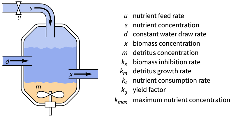
nssm = NonlinearStateSpaceModel[IconizedObject[«eqns»], {{x[t], Subscript[x, 0]}, {s[t], Subscript[s, 0]}, {m[t], Subscript[m, 0]}}, u[t], x[t], t] /. IconizedObject[«pars»]StateResponse[{nssm, {0.75, 0.01, 2}}, 0, {t, 0, 60}];
Plot[%, {t, 0, 60}, PlotRange -> All, PlotLegends -> {x, s, m}]sspec = <|"InputModel" -> nssm, "TrackedOutputs" -> 1|>;wts = {DiagonalMatrix[{10, 1, 1, 10^2}], {{300}}};
τ = 0.2;dlqr = DiscreteLQRegulatorGains[sspec, wts, τ, "Data"]dcsys = dlqr["DiscreteTimeClosedLoopSystem"]一定のバイオマス濃度1.25を追跡して系のシミュレーションを行う:
Subscript[x, ref] = 1.25;sr = StateResponse[{dcsys, {0.75, 0, 2}}, Table[Subscript[x, ref], 300]];ListStepPlot[sr[[1]], IconizedObject[«plotOpts»]]cm = dlqr["DiscreteTimeControllerModel"]cinps = Join[{Table[Subscript[x, ref], 300], sr[[1]]}, sr[[1 ;; 3]]];
ListStepPlot[OutputResponse[cm, cinps], PlotRange -> All]電気系 (1)
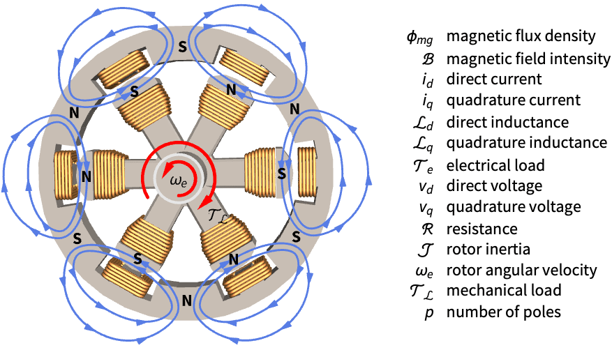
pmsm = NonlinearStateSpaceModel[IconizedObject[«eqns»] /. IconizedObject[«pars»], {Subscript[i, d][t], Subscript[i, q][t], Subscript[ω, e][t]}, {Subscript[v, d][t], Subscript[v, q][t], Subscript[𝒯, ℒ][t]}, Subscript[ω, e][t], t]//SimplifyOutputResponse[pmsm, {0, 0, UnitStep[t - 1]}, {t, 0, 1500}];
Plot[%, {t, 0, 1500}, PlotRange -> All]sspec = <|"InputModel" -> pmsm, "FeedbackInputs" -> {1, 2}|>;最大制御努力の24vについて,サンプリング周期と制御重みの集合を指定する:
τ = (1/60.0);
wts = {DiagonalMatrix[{1, 1, 1000}], DiagonalMatrix[{(1/24^2), (1/24^2)}]};dlqr = DiscreteLQRegulatorGains[sspec, wts, τ, "Data"]dcsys = dlqr["DiscreteTimeClosedLoopSystem"]//Chop閉ループ系がステップ入力外乱に安定するまでに5秒ほどかかる:
sr = StateResponse[dcsys, Table[{0, 0, 1}, 1000]];
ListStepPlot[sr[[3]], DataRange -> {0, 999 τ}, PlotRange -> All]cm = dlqr["DiscreteTimeControllerModel"]OutputResponse[cm, Join[Table[{0, 0}, 1000], sr]];
ListStepPlot[%, DataRange -> {0, 999 τ}, IconizedObject[«plotOpts»]]海洋系 (1)
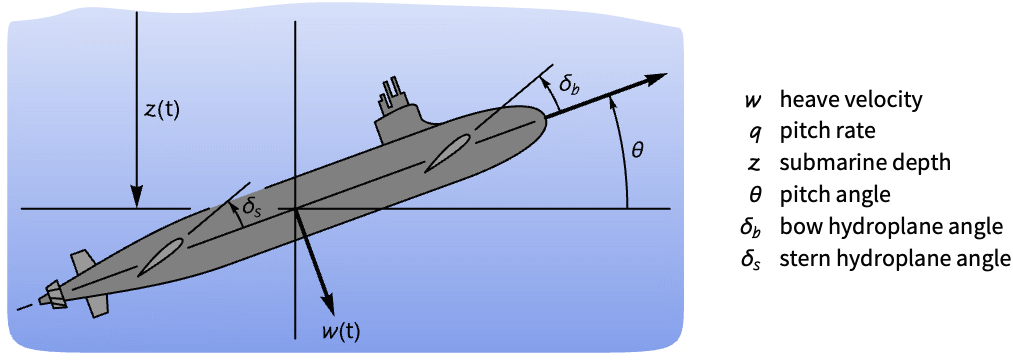
submarine = StateSpaceModel[IconizedObject[«abcd»], IconizedObject[«labels»]]コントローラがないと,潜水艦のピッチと深度は状態の外乱に対して不安定である:
OutputResponse[{submarine, {1, 0, 0.5, 0.2}}, {0, 0}, {t, 0, 20}];
Table[Plot[ℴ𝓇[[1]], {t, 0, 20}, IconizedObject[«plotOpts»]], {ℴ𝓇, ({%, {𝓏, θ}})}]深度
とピッチ
を設定する.これは追跡される出力としての出力1および2である:
sspec = <|"InputModel" -> submarine, "TrackedOutputs" -> {1, 2}|>;wts = {DiagonalMatrix[{5, 5, 10, 10, 10^3, 10^3}], 10^3IdentityMatrix[2]};
τ = 0.2;dlqr = DiscreteLQRegulatorGains[sspec, wts, τ, "Data"]dcsys = dlqr["DiscreteTimeClosedLoopSystem"]sr = StateResponse[dcsys, Table[{-10, 0}, 750]];
Table[ListStepPlot[𝓈𝓇[[1]], IconizedObject[«plotOpts»]], {𝓈𝓇, ({sr[[3 ;; 4]], {𝓏, θ}})}]cm = dlqr["DiscreteTimeControllerModel"]cinps = Join[Table[{-10, 0}, 750], sr[[{3, 4, 1, 2, 3, 4}]]];ListStepPlot[OutputResponse[cm, cinps], IconizedObject[«plotOpts»]]特性と関係 (5)
DiscreteLQRegulatorGainsは,エミュレートされた離散時間系のゲインとして計算される:
ssm = StateSpaceModel[{a = (| | |
| - | --- |
| 0 | 1 |
| 0 | -10 |), b = (| |
| - |
| 0 |
| 1 |), c = (1 0)}]{{q, r}, τ} = {{(| | |
| -- | - |
| 10 | 0 |
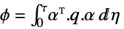
| 0 | 0 |), (1)}, 0.1};ssmd = ToDiscreteTimeModel[ssm, τ, Method -> "ZeroOrderHold"]ϕ = Subsuperscript[∫, 0, τ]MatrixExp[a t].q.MatrixExp[a t]ⅆtρ = Subsuperscript[∫, 0, τ](r + (Subsuperscript[∫, 0, t]MatrixExp[a η].bⅆη).q.Subsuperscript[∫, 0, t]MatrixExp[a η].bⅆη)ⅆtψ = Subsuperscript[∫, 0, τ]MatrixExp[a t].q.(Subsuperscript[∫, 0, t]MatrixExp[a η].bⅆη) ⅆtLQRegulatorGains[ssmd, {ϕ, ρ, ψ}]DiscreteLQRegulatorGainsは同じ結果を与える:
DiscreteLQRegulatorGains[ssm, {q, r}, τ]eqns = {Derivative[1][Subscript[x, 1]][t] == Subscript[x, 2][t], u[t] == -2 Subscript[x, 1][t] + Subscript[x, 2][t] + Derivative[1][Subscript[x, 2]][t]};
states = {Subscript[x, 1][t], Subscript[x, 2][t]};ssm = StateSpaceModel[eqns, states, u[t], Subscript[x, 1][t], t]τ = 0.4;
cd = DiscreteLQRegulatorGains[ssm, {(| | |
| - | - |
| 1 | 0 |
| 0 | 1 |), {{1}}}, τ, "Data"]dcsys = cd["DiscreteTimeClosedLoopSystem"]sr = StateResponse[{dcsys, {1, -1}}, Table[0, 10 / τ]];
p = ListStepPlot[%, IconizedObject[«plotOpts»]]fb = WhenEvent@@{Mod[t, τ] == 0, u[t] -> First[-cd["FeedbackGains"].states]}ceqns = Join[eqns, {Subscript[x, 1][0] == 1, Subscript[x, 2][0] == -1, u[0] == 0}, {fb}]NDSolve[ceqns, Join[states, {u[t]}], {t, 0, 7}, DiscreteVariables -> u[t]];
csols = First[states /. %]Legended[Show[Plot[csols, {t, 0, 7}, IconizedObject[«plotOpts»]], p], IconizedObject[«lineLegend»]]サンプリング周期を下げるとサンプルされたデータの系がよりよく近似できる:
τ = {0.4, 0.1, 0.025};さまざまな
の値についての離散時間閉ループ系とフィードバックゲイン:
{dcsys, κ} = Table[DiscreteLQRegulatorGains[IconizedObject[«ssm»], IconizedObject[«wts»], i, IconizedObject[«props»]], {i, τ}];Grid[{dcsys, κ}, IconizedObject[«gridOpts»]]sr = Table[StateResponse[{dcsys[[i]], {1, -1}}, Table[0, 8 / τ[[i]]]], {i, 3}];
p = Table[ListStepPlot[sr[[i, k]], DataRange -> {0, 8}, IconizedObject[«plotOpts»]], {i, 3}, {k, 2}]sols = Table[NDSolve[{IconizedObject[«ssmEqns»], Subscript[x, 1][0] == 1, Subscript[x, 2][0] == -1, u[0] == 0, WhenEvent[Mod[t, τ[[i]]] == 0, u[t] -> -First[κ[[i]].IconizedObject[«states»]]]}, Join[IconizedObject[«states»], {u[t]}], {t, 0, 8}, DiscreteVariables -> u[t]], {i, 3}];Shallow[xSols = Table[First[IconizedObject[«states»] /. %[[i]]], {i, 3}]]サンプリング周期が短くなるにつれて,系の応答間の相違も小さくなる:
Table[Legended[Show[Plot[Evaluate@xSols[[i, k]], {t, 0, 8}, IconizedObject[«plotOpts»]], p[[i, k]]], IconizedObject[«leg»]], {i, 3}, {k, 2}];
Grid[%, Spacings -> {2.5, 1}]サンプリング周期を短くすると,サンプルデータの系の制御努力の近似がよりよくなる:
τ = {0.4, 0.1, 0.025};Short[sr = IconizedObject[«sr»]]Short[sols = IconizedObject[«sols»]]dcm = Table[DiscreteLQRegulatorGains[IconizedObject[«ssm»], IconizedObject[«wts»], i, "DiscreteTimeControllerModel"], {i, τ}]ce = Table[OutputResponse[dcm[[i]], Join[{Table[0, 8 / τ[[i]]]}, sr[[i]]]], {i, 3}];
p = Table[ListStepPlot[ce[[i]], DataRange -> {0, 8}, IconizedObject[«plotOpts»]], {i, 3}]csols = Table[First[{u[t]} /. sols[[i]]], {i, 3}]サンプリング周期が短くなると,系の制御努力間の違いも小さくなる:
Grid[{Table[Legended[Show[Plot[csols[[i]], {t, 0, 8}, IconizedObject[«plotOpts»]], p[[i]]], IconizedObject[«leg»]], {i, 3}]}, Spacings -> 2]サンプリング周期を短くすると閉ループ極が単位円に近くなる,つまり不安定になる:
τ = {0.4, 0.1, 0.025};dcsys = Table[DiscreteLQRegulatorGains[IconizedObject[«ssm»], IconizedObject[«wts»], i, "DiscreteTimeClosedLoopSystem"], {i, τ}]Table[Eigenvalues@First@Normal[dcsys[[i]]], {i, 3}];
Grid[{{"τ = 0.4", "τ = 0.1", "τ = 0.025"}, %}, IconizedObject[«gridOpts»]]考えられる問題 (1)
ssm = StateSpaceModel[{{{-3, 1}, {0, 2}}, {{1}, {0}}, {{1, 0}, {0, 1}}, {{0}, {0}}},
SamplingPeriod -> None, SystemsModelLabels -> None];DiscreteLQRegulatorGains[ssm, {(| | |
| - | -- |
| 1 | 0 |
| 0 | 1. |), (1)}, 1]不安定な極2が制御不可能なので,この系は安定かされていない:
Table[{λ, ControllableModelQ[{ssm, λ}]}, {λ, Eigenvalues[Normal[ssm][[1]]]}]関連するガイド
-
▪
- 状態空間モデルを使った設計 ▪
- 制御系
テキスト
Wolfram Research (2010), DiscreteLQRegulatorGains, Wolfram言語関数, https://reference.wolfram.com/language/ref/DiscreteLQRegulatorGains.html (2021年に更新).
CMS
Wolfram Language. 2010. "DiscreteLQRegulatorGains." Wolfram Language & System Documentation Center. Wolfram Research. Last Modified 2021. https://reference.wolfram.com/language/ref/DiscreteLQRegulatorGains.html.
APA
Wolfram Language. (2010). DiscreteLQRegulatorGains. Wolfram Language & System Documentation Center. Retrieved from https://reference.wolfram.com/language/ref/DiscreteLQRegulatorGains.html
BibTeX
@misc{reference.wolfram_2026_discretelqregulatorgains, author="Wolfram Research", title="{DiscreteLQRegulatorGains}", year="2021", howpublished="\url{https://reference.wolfram.com/language/ref/DiscreteLQRegulatorGains.html}", note=[Accessed: 15-September-2026]}
BibLaTeX
@online{reference.wolfram_2026_discretelqregulatorgains, organization={Wolfram Research}, title={DiscreteLQRegulatorGains}, year={2021}, url={https://reference.wolfram.com/language/ref/DiscreteLQRegulatorGains.html}, note=[Accessed: 15-September-2026]}