DiscreteLQRegulatorGains[sspec,wts,τ]
给出离散时间状态反馈增益矩阵,其中,对于最小化权重为 wts 的成本函数的连续时间系统指定 sspec,采样周期为 τ.
DiscreteLQRegulatorGains[…,"prop"]
给出属性 "prop" 的值.
DiscreteLQRegulatorGains

DiscreteLQRegulatorGains[sspec,wts,τ]
给出离散时间状态反馈增益矩阵,其中,对于最小化权重为 wts 的成本函数的连续时间系统指定 sspec,采样周期为 τ.
DiscreteLQRegulatorGains[…,"prop"]
给出属性 "prop" 的值.
更多信息和选项
- DiscreteLQRegulatorGains 亦称为离散线性二次调节器、离散线性二次成本等效调节器或离散线性二次仿真调节器.

- DiscreteLQRegulatorGains 通常用于计算调节控制器或跟踪控制器的数字化实现.
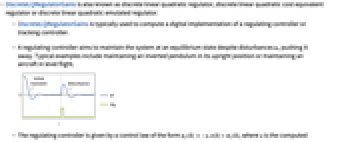
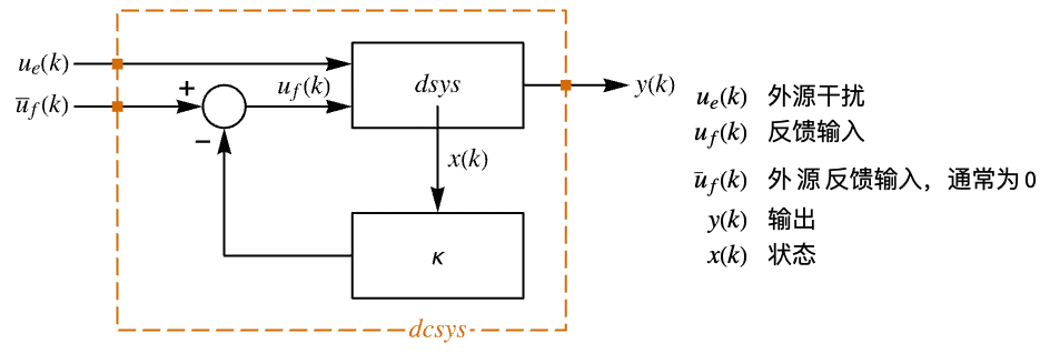
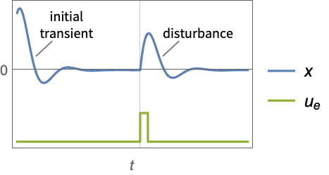
- 调节控制器旨在尽管有
干扰的情况下仍将系统保持在平衡状态. 典型范例包括将倒立摆保持在直立位置或保持飞机水平飞行. - 调节控制器由

的控制律给出,其中
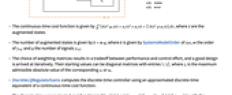
是计算得到的增益矩阵. - 连续时间成本函数由
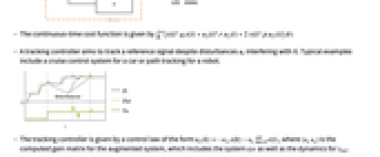
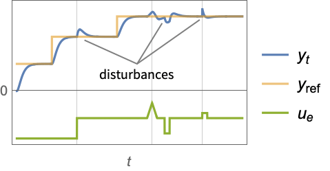
给出. - 跟踪控制器旨在有扰动
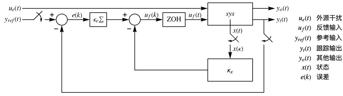
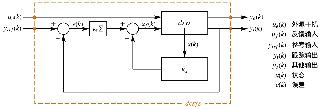
干扰的情况下跟踪参考信号. 典型范例包括汽车的巡航控制系统或机器人的路径跟踪. - 跟踪控制器由形式为

的控制律给出,其中
是计算出的增强系统的增益矩阵,包括系统 sys 和
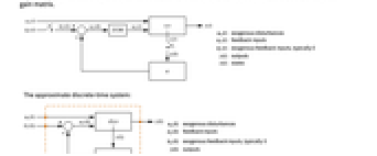
的动力. - 近似离散时间系统:
- 连续时间成本函数由
给出,其中
为增强状态. - 增强状态的数量由
给出,其中
由 sys 的 SystemsModelOrder 给出、
由 yref 的阶给出、
由 yref 的信号数给出. - 权重矩阵的选择需要性能和控制工作量之间的平衡,通过迭代可以获取比较理想的设计. 它们的起始值可以是有项
的对角矩阵,其中 zi 是相应的 xi 或 ui 的最大允许绝对值. - DiscreteLQRegulatorGains 使用连续时间成本函数的近似离散时间等效值计算离散时间控制器.
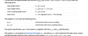
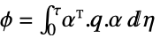
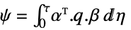
- 离散时间近似成本函数是
,具有以下项: -
状态权重矩阵 
输入权重矩阵 
交叉耦合权重矩阵 
状态向量
用于调节且
用于追踪 - 权重 wts 可采用以下形式:
-
{q,r} 没有交叉耦合的成本函数 {q,r,p} 含有交叉耦合矩阵 p 的成本函数 - 系统规约 sspec 是系统 sys 与 uf、yt 和 yref 规约.
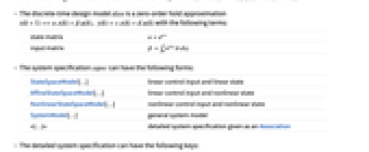
- 系统 sys 可以 StateSpaceModel[{a,b,c,d}] 形式给出,其中 a, b, c 和 d 分别表示状态、输入、输出和连续时间系统中的馈通矩阵

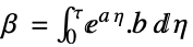
. - 离散时间设计模型 dsys 为保持零阶的近似形式
,有如下项: -
状态矩阵 
输入矩阵 
- 系统指定 sspec 可采用以下形式:
-
StateSpaceModel[…] 线性控制输入和线性状态 AffineStateSpaceModel[…] 线性控制输入和非线性状态 NonlinearStateSpaceModel[…] 非线性控制输入和非线性状态 SystemModel[…] 一般系统模型 <|…|> 用 Association 给出的详细系统指定 - 详细系统指定中可含有以下键:
-
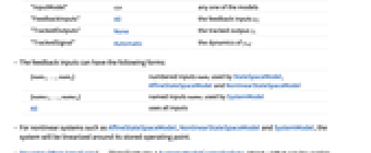
"InputModel" sys 任意一个模型 "FeedbackInputs" All 反馈输入 uf "TrackedOutputs" None 跟踪输出 yt "TrackedSignal" Automatic yref 的动力 - 反馈输入可采用以下形式:
-
{num1,…,numn} 由 StateSpaceModel、AffineStateSpaceModel 和 NonlinearStateSpaceModel 使用的编号输入 numi {name1,…,namen} 由 SystemModel 使用的编号输入 namei All 使用所有输入 - 对于非线性系统,如 AffineStateSpaceModel、NonlinearStateSpaceModel 和 SystemModel,系统将围绕其存储的工作点进行线性化.
- DiscreteLQRegulatorGains[…,"Data"] 返回一个 SystemsModelControllerData 对象 cd,可通过 cd["prop"] 提取其他属性.
- 可用 DiscreteLQRegulatorGains[…,"prop"] 直接给出 cd["prop"] 的值.
- 属性 "prop" 可取的值包括:
-
"BlockDiagram" csys 的采样数据框图 "ClosedLoopSystem" csys 的采样数据闭环系统 {"ClosedLoopSystem",cspec} 对 csys 形式的详细控制 "Design" 控制器设计的类型 "DesignModel" 设计所用的模型 "DiscreteTimeBlockDiagram" dcsys 的框图 "DiscreteTimeClosedLoopPoles" "DiscreteTimeClosedLoopSystem" 的极点 "DiscreteTimeClosedLoopSystem" dcsys {"DiscreteTimeClosedLoopSystem",cspec} 是否合并离散时间闭环系统 dsys "DiscreteTimeControllerModel" dcm "DiscreteTimeDesignModel" 近似离散时间模型 dsys "DiscreteTimeFeedbackGainsModel" dgm 或 {dgm1,dgm2} "DiscreteTimeOpenLoopPoles" dsys 的极点 "DiscreteTimeWeights" 近似成本函数的权重 ϕ、ρ、π "FeedbackGains" 增益矩阵 κ 或其等价物 "FeedbackInputs" 用 sys 的 uf 作为反馈 "InputCount" sys 的输入 u 的个数 "InputModel" 输入模型 sys "OpenLoopPoles" "DesignModel" 的极点 "OutputCount" sys 的输出 y 的个数 "SamplingPeriod" 采样 period τ "StateCount" sys 的状态 x 的数量 "TrackedOutputs" 被跟踪的 sys 的输出 yt - cspec 的密钥包括:
-
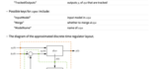
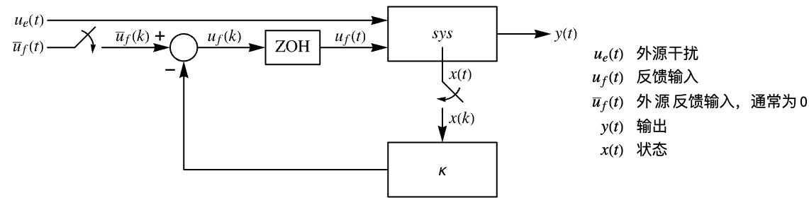
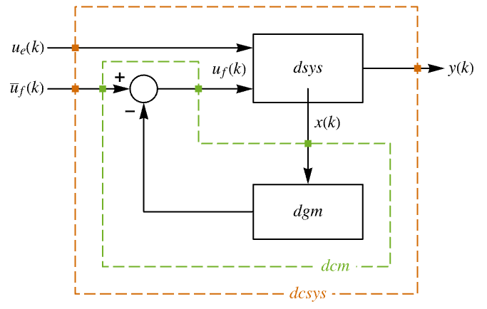
"InputModel" csys 中的输入模型 "Merge" 是否合并 csys "ModelName" csys 的名称 - 近似离散时间调节器布局图.
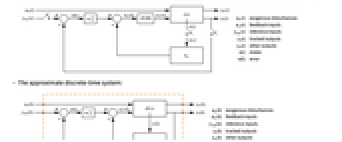
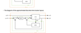
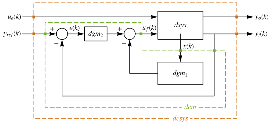
- 近似离散时间跟踪器布局图.
范例
打开所有单元 关闭所有单元基本范例 (4)
具有反馈输入 uf 和外生输入 ue 的系统的系统规范 sspec:
sspec = <|"InputModel" -> StateSpaceModel[{{{2, 1}, {4, -5}}, {{1, 0}, {0, 0.1}}, {{1, 0}}, {{0, 0}}},
SamplingPeriod -> None, SystemsModelLabels ->
{{Subscript[u, f], Subscript[u, e]}}], "FeedbackInputs" -> 1|>;wts = {(| | |
| -- | -- |
| 10 | 0 |
| 0 | 10 |), {{0.1}}};
τ = 0.5;DiscreteLQRegulatorGains[sspec, wts, τ]nssm = NonlinearStateSpaceModel[{{-1 + 3*Subscript[x, 2],
u + 2*Subscript[x, 1] - Subscript[x, 2]},
{Subscript[x, 1] + Subscript[x, 2]}},
{{Subscript[x, 1], 0}, {Subscript[x, 2], 1}}, {{u, 1}},
{Automatic}, Automatic, SamplingPeriod -> None];wts = {(| | |
| - | - |
| 1 | 0 |
| 0 | 1 |), {{0.25}}};
τ = 0.2;DiscreteLQRegulatorGains[nssm, wts, τ]sspec = <|"InputModel" -> StateSpaceModel[{{{3, 0}, {-1, 5}}, {{0, 1}, {1, 0}}, {{1, 0}}, {{0, 0}}}, SamplingPeriod -> None,
SystemsModelLabels -> None], "TrackedOutputs" -> 1|>;wts = {(| | | |
| -- | ---- | -- |
| 10 | 0 | 0 |
| 0 | 10^2 | 0 |
| 0 | 0 | 10 |), (| | |
| - | - |
| 1 | 0 |
| 0 | 1 |)};
τ = 0.1;DiscreteLQRegulatorGains[sspec, wts, τ]ssm = StateSpaceModel[{{{0., 1.}, {-6., 5.}}, {{0.}, {1.}}, {{1, 0}}, {{0.}}}, SamplingPeriod -> None,
SystemsModelLabels -> None];wts = {(| | |
| - | - |
| 1 | 0 |
| 0 | 1 |), {{0.25}}};
τ = 0.2;dlqr = DiscreteLQRegulatorGains[ssm, wts, τ, "Data"]{olPoles, clPoles} = dlqr[{"OpenLoopPoles", "DiscreteTimeClosedLoopPoles"}]PoleZeroPlot[dlqr["InputModel"]]PoleZeroPlot[dlqr["DiscreteTimeClosedLoopSystem"]]范围 (30)
基本用法 (7)
ssm = StateSpaceModel[{{{-1}}, {{1}}}, SamplingPeriod -> None, SystemsModelLabels -> None];κ = DiscreteLQRegulatorGains[ssm, {{{1}}, {{1}}}, 0.1]dssm = Table[ToDiscreteTimeModel[ssm, τ, Method -> "ZeroOrderHold"], {τ, vl}]SystemsModelStateFeedbackConnect[dssm, κ]ssm = StateSpaceModel[{{{-1}}, {{1}}}, SamplingPeriod -> None, SystemsModelLabels -> None];κ = DiscreteLQRegulatorGains[ssm, {{{1}}, {{1}}}, 0.1]dssm = ToDiscreteTimeModel[ssm, 0.1, Method -> "ZeroOrderHold"]SystemsModelStateFeedbackConnect[dssm, κ]ssm = StateSpaceModel[{{{-1}}, {{1}}}, SamplingPeriod -> None, SystemsModelLabels -> None];
vl = {0.01, 0.1, 1.0};κ = Table[DiscreteLQRegulatorGains[ssm, {{{1}}, {{1}}}, τ], {τ, vl}]dssm = Table[ToDiscreteTimeModel[ssm, τ, Method -> "ZeroOrderHold"], {τ, vl}]MapThread[SystemsModelStateFeedbackConnect, {dssm, κ}]ssm = StateSpaceModel[{{{-3, 0}, {0, -1}}, {{0.5}, {-0.5}}, {{-1, -1}}, {{0}}}, SamplingPeriod -> None,
SystemsModelLabels -> None];κ = DiscreteLQRegulatorGains[ssm, {(| | |
| - | - |
| 5 | 0 |
| 0 | 5 |), (1)}, 0.5]Dimensions[κ]{SystemsModelDimensions[ssm][[1]], SystemsModelOrder[ssm]}ssm = StateSpaceModel[{{{0, 0, -5}, {1, 0, -9.5}, {0, 1, -5.5}}, {{-5, 1}, {-4.5, 0}, {-1, 0}},
{{0, 0, 1}}, {{1, 0}}}, SamplingPeriod -> None, SystemsModelLabels -> None];MatrixForm[κ1 = DiscreteLQRegulatorGains[ssm, {(| | | |
| - | - | - |
| 1 | 0 | 0 |
| 0 | 1 | 0 |
| 0 | 0 | 1 |), (| | |
| - | - |
| 1 | 0 |
| 0 | 2 |)}, 0.1]]MatrixForm[κ2 = DiscreteLQRegulatorGains[ssm, {(| | | |
| - | - | - |
| 1 | 0 | 0 |
| 0 | 1 | 0 |
| 0 | 0 | 1 |), (| | |
| - | - |
| 2 | 0 |
| 0 | 1 |)}, 0.1]]Norm /@ κ1
Norm /@ κ2Norm /@ DiscreteLQRegulatorGains[ssm, {(| | | |
| - | - | - |
| 1 | 0 | 0 |
| 0 | 1 | 0 |
| 0 | 0 | 1 |), (| | |
| -- | - |
| 10 | 0 |
| 0 | 1 |)}, 0.1]ssm = StateSpaceModel[{{{1, 0, 0}, {0, -2, 0}, {0, 0, 3}}, {{0, 0, -1}, {1, 0, -2}, {0.1, 0, 0.5}},
{{1, 0, 0}}, {{0, 0, 0}}}, SamplingPeriod -> None, SystemsModelLabels -> None];
MatrixForm[DiscreteLQRegulatorGains[ssm, {(| | | |
| -- | --- | - |
| 10 | 0 | 0 |
| 0 | 0.1 | 0 |
| 0 | 0 | 1 |), (| | | |
| - | - | - |
| 1 | 0 | 0 |
| 0 | 1 | 0 |
| 0 | 0 | 1 |), (| | | |
| - | - | - |
| 1 | 2 | 0 |
| 2 | 0 | 0 |
| 0 | 1 | 1 |)}, 1]]nssm = NonlinearStateSpaceModel[{{x2, u*(1 + x1) +
x1*x2 + Cos[x1]}, {x1}},
{{x1, 0}, {x2, -1}}, {{u, -1}}, {Automatic}, Automatic,
SamplingPeriod -> None];DiscreteLQRegulatorGains[nssm, {(| | |
| - | - |
| 1 | 0 |
| 0 | 1 |), (1)}, 0.1]ssm = StateSpaceModel[nssm];DiscreteLQRegulatorGains[ssm, {(| | |
| - | - |
| 1 | 0 |
| 0 | 1 |), (1)}, 0.1]工厂模型 (5)
DiscreteLQRegulatorGains[StateSpaceModel[{{{0, 1, 0}, {0, 0, 1}, {5, 9, 3}}, {{0}, {0}, {1}}, {{8, 2, 1}}, {{0}}},
SamplingPeriod -> None, SystemsModelLabels -> None], {(| | | |
| - | -- | -- |
| 1 | 0 | 0 |
| 0 | 10 | 0 |
| 0 | 0 | 10 |), (1)}, 0.1]描述符 StateSpaceModel:
DiscreteLQRegulatorGains[StateSpaceModel[{{{-0.3, 0.65, 0}, {0, 1, 0}, {0.25, -0.5, -0.6}}, {{-1}, {0.5}, {0.7}},
{{1, 0, 0}}, {{0}}, {{3, 0, 0}, {5, 0, 0}, {0, 1, 0}}}, SamplingPeriod -> None,
SystemsModelLabels -> None], {(| | | |
| - | - | - |
| 4 | 0 | 0 |
| 0 | 3 | 0 |
| 0 | 0 | 5 |), (1)}, .1]DiscreteLQRegulatorGains[AffineStateSpaceModel[{{Sin[Subscript[x, 1]] + Subscript[x, 2],
-Subscript[x, 1] - Subscript[x, 2]},
{{Subscript[x, 1]}, {1}}, {Subscript[x, 1]}, {{0}}},
{Subscript[x, 1], Subscript[x, 2]}, {{u, 0}}, {Automatic},
Automatic, SamplingPeriod -> None], {(| | |
| - | - |
| 1 | 0 |
| 0 | 1 |), (1)}, 0.1]DiscreteLQRegulatorGains[NonlinearStateSpaceModel[
{{Subscript[x, 2] + Subscript[x, 1]*Subscript[x, 2],
u + Subscript[x, 1]}, {Subscript[x, 1]}},
{Subscript[x, 1], Subscript[x, 2]}, {u}, {Automatic},
Automatic, SamplingPeriod -> None], {(| | |
| - | - |
| 1 | 0 |
| 0 | 1 |), (1)}, 0.1]sm = CreateSystemModel[{x''[t] + x'[t] + x[t] == u[t], y[t] == x[t]}, t, {"u"∈"Modelica.Blocks.Interfaces.RealInput", "y"∈"Modelica.Blocks.Interfaces.RealOutput"}];DiscreteLQRegulatorGains[sm, {(| | |
| - | - |
| 1 | 0 |
| 0 | 1 |), (1)}, 0.1]属性 (14)
默认情况下,DiscreteLQRegulatorGains 返回离散时间反馈增益:
DiscreteLQRegulatorGains[StateSpaceModel[{{{0, 1}, {-1, -2}}, {{0}, {1}}, {{1, 0}}, {{0}}}, SamplingPeriod -> None,
SystemsModelLabels -> None], {(| | |
| - | - |
| 1 | 0 |
| 0 | 1 |), (1)}, 1.0]% == DiscreteLQRegulatorGains[StateSpaceModel[{{{0, 1}, {-1, -2}}, {{0}, {1}}, {{1, 0}}, {{0}}}, SamplingPeriod -> None,
SystemsModelLabels -> None], {(| | |
| - | - |
| 1 | 0 |
| 0 | 1 |), (1)}, 1.0, "FeedbackGains"]κ = DiscreteLQRegulatorGains[NonlinearStateSpaceModel[
{{-Subscript[x, 1] + u*Subscript[x, 1] +
Subscript[x, 2]/E^Subscript[x, 1],
E^Subscript[x, 2] - Subscript[x, 1]}, {Subscript[x, 2]}},
{{Subscript[x, 1], 1}, {Subscript[x, 2], 0}}, {{u, 1.}},
{Automatic}, Automatic, SamplingPeriod -> None], {(| | |
| - | - |
| 1 | 0 |
| 0 | 1 |), (1)}, 1.0]{κ0, κ1} = {κ /. {Subscript[x, _] -> 0}, D[κ, {{Subscript[x, 1], Subscript[x, 2]}}]}DiscreteLQRegulatorGains[StateSpaceModel[{{{0, 1}, {-1, -2}}, {{0}, {1}}, {{1, 0}}, {{0}}}, SamplingPeriod -> None,
SystemsModelLabels -> None], {(| | |
| - | - |
| 1 | 0 |
| 0 | 1 |), (1)}, 1.0, "DiscreteTimeFeedbackGainsModel"]DiscreteLQRegulatorGains[NonlinearStateSpaceModel[{{Subscript[x, 2], -2/3 + u -
Subscript[x, 1]/3 - Subscript[x, 2]/2},
{Subscript[x, 1]}}, {{Subscript[x, 1], 1},
{Subscript[x, 2], 0}}, {{u, 1.}}, {Automatic}, Automatic,
SamplingPeriod -> None], {(| | |
| - | - |
| 1 | 0 |
| 0 | 1 |), (1)}, 1.0, "DiscreteTimeFeedbackGainsModel"]DiscreteLQRegulatorGains[StateSpaceModel[{{{0., 1.}, {-0.05, -0.9}}, {{0}, {1}}, {{1, 0}}, {{0}}},
{Subscript[x, 1], Subscript[x, 2]}, {{f, 0}},
SamplingPeriod -> None, SystemsModelLabels -> None], {(| | |
| - | - |
| 1 | 0 |
| 0 | 1 |), (1)}, 1.0, "DiscreteTimeClosedLoopSystem"]DiscreteLQRegulatorGains[StateSpaceModel[{{{0., 1.}, {-0.05, -0.9}}, {{0}, {1}}, {{1, 0}}, {{0}}},
{Subscript[x, 1], Subscript[x, 2]}, {{f, 0}},
SamplingPeriod -> None, SystemsModelLabels -> None], {(| | |
| - | - |
| 1 | 0 |
| 0 | 1 |), (1)}, 1.0, "DiscreteTimeBlockDiagram"]DiscreteLQRegulatorGains[StateSpaceModel[{{{0., 1.}, {-0.05, -0.9}}, {{0}, {1}}, {{1, 0}}, {{0}}},
{Subscript[x, 1], Subscript[x, 2]}, {{f, 0}},
SamplingPeriod -> None, SystemsModelLabels -> None], {(| | |
| - | - |
| 1 | 0 |
| 0 | 1 |), (1)}, 1.0, "ClosedLoopSystem"]DiscreteLQRegulatorGains[StateSpaceModel[{{{0., 1.}, {-0.05, -0.9}}, {{0}, {1}}, {{1, 0}}, {{0}}},
{Subscript[x, 1], Subscript[x, 2]}, {{f, 0}},
SamplingPeriod -> None, SystemsModelLabels -> None], {(| | |
| - | - |
| 1 | 0 |
| 0 | 1 |), (1)}, 1.0, "BlockDiagram"]assm = AffineStateSpaceModel[{{Subscript[x, 2], -0.05*Subscript[x, 1] -
0.9*Subscript[x, 2]^2}, {{0}, {1}}, {Subscript[x, 1]}, {{0}}},
{Subscript[x, 1], Subscript[x, 2]}, {{f, 0}}, {Automatic},
Automatic, SamplingPeriod -> None];
{wts, τ} = {{(| | |
| - | - |
| 1 | 0 |
| 0 | 1 |), (1)}, 1.0};DiscreteLQRegulatorGains[assm, wts, τ, "DiscreteTimeClosedLoopPoles"]DiscreteLQRegulatorGains[assm, {10wts[[1]], wts[[2]]}, τ, "DiscreteTimeClosedLoopPoles"]DiscreteLQRegulatorGains[assm, {wts[[1]], 10wts[[2]]}, τ, "DiscreteTimeClosedLoopPoles"]assm = AffineStateSpaceModel[{{Subscript[x, 2], -0.05*Subscript[x, 1] -
0.9*Subscript[x, 2]^2}, {{0}, {1}}, {Subscript[x, 1]}, {{0}}},
{Subscript[x, 1], Subscript[x, 2]}, {{f, 0}}, {Automatic},
Automatic, SamplingPeriod -> None];
{wts, τ} = {{(| | |
| - | - |
| 1 | 0 |
| 0 | 1 |), (1)}, 1.0};DiscreteLQRegulatorGains[assm, wts, τ, "DesignModel"]DiscreteLQRegulatorGains[assm, wts, τ, "OpenLoopPoles"]DiscreteLQRegulatorGains[assm, wts, τ, "DiscreteTimeDesignModel"]DiscreteLQRegulatorGains[assm, wts, τ, "DiscreteTimeOpenLoopPoles"]DiscreteLQRegulatorGains[AffineStateSpaceModel[{{Subscript[x, 2], -0.05*Subscript[x, 1] -
0.9*Subscript[x, 2]^2}, {{0}, {1}}, {Subscript[x, 1]}, {{0}}},
{Subscript[x, 1], Subscript[x, 2]}, {{f, 0}}, {Automatic},
Automatic, SamplingPeriod -> None], {(| | |
| - | - |
| 1 | 0 |
| 0 | 1 |), (1)}, 1.0, "DiscreteTimeWeights"];MatrixForm /@ %DiscreteLQRegulatorGains[AffineStateSpaceModel[{{Subscript[x, 2], -0.05*Subscript[x, 1] -
0.9*Subscript[x, 2]^2}, {{0}, {1}}, {Subscript[x, 1]}, {{0}}},
{Subscript[x, 1], Subscript[x, 2]}, {{f, 0}}, {Automatic},
Automatic, SamplingPeriod -> None], {(| | |
| - | - |
| 1 | 0 |
| 0 | 1 |), (1)}, 1.0, "Design"]Dataset[Table[{prop, DiscreteLQRegulatorGains[IconizedObject[«sys»], IconizedObject[«wts»], 1.0, prop]}, {prop, IconizedObject[«props»]}]]𝒸𝒹 = DiscreteLQRegulatorGains[IconizedObject[«sspec»], IconizedObject[«wts»], 1.0, "Data"]𝒸𝒹["Properties"]𝒸𝒹["DiscreteTimeClosedLoopPoles"]跟踪 (4)
sspec = <|"InputModel" -> StateSpaceModel[{{{0, 7}, {-1, -6}}, {{0}, {1}}, {{5, 0}}, {{0}}}, SamplingPeriod -> None,
SystemsModelLabels -> None], "TrackedOutputs" -> 1|>;𝒸𝒹 = DiscreteLQRegulatorGains[sspec, {(| | | |
| --- | - | --- |
| 100 | 0 | 0 |
| 0 | 1 | 0 |
| 0 | 0 | 0.5 |), (1)}, 0.75, "Data"]OutputResponse[𝒸𝒹["DiscreteTimeClosedLoopSystem"], ref = Table[1, 30]];
ListStepPlot[{ref, %[[1]]}, IconizedObject[«plotOpts»]]𝒸𝒹["DiscreteTimeBlockDiagram"]sspec = <|"InputModel" -> StateSpaceModel[{{{2., 0}, {0, -2}}, {{1., 0}, {0, 1}}, {{1, 0}, {3., 1}}, {{0, 0}, {0, 0}}},
SamplingPeriod -> None, SystemsModelLabels -> None], "TrackedOutputs" -> {1, 2}|>;𝒸𝒹 = DiscreteLQRegulatorGains[sspec, {(| | | | |
| - | - | --- | --- |
| 1 | 0 | 0 | 0 |
| 0 | 1 | 0 | 0 |
| 0 | 0 | 100 | 0 |
| 0 | 0 | 0 | 100 |), (| | |
| - | - |
| 1 | 0 |
| 0 | 1 |)}, 0.75, "Data"]refs = Table[ConstantArray[RandomInteger[{-12, -4}], 30], 2];
or = OutputResponse[𝒸𝒹["DiscreteTimeClosedLoopSystem"], refs];ListStepPlot[Riffle[refs, or], IconizedObject[«plotOpts»]]sspec = <|"InputModel" -> StateSpaceModel[{{{0, 1}, {-5, -3}}, {{0}, {1}}, {{5, 0}}, {{0}}}, SamplingPeriod -> None,
SystemsModelLabels -> None], "TrackedOutputs" -> 1|>;𝒸𝒹 = DiscreteLQRegulatorGains[sspec, {(| | | |
| -- | - | -- |
| 10 | 0 | 0 |
| 0 | 1 | 0 |
| 0 | 0 | 10 |), {{1}}}, 1.0, "Data"]cm = 𝒸𝒹["DiscreteTimeControllerModel"]ref = Table[1, 30]dcsys = 𝒸𝒹["DiscreteTimeClosedLoopSystem"];Short[sr = StateResponse[dcsys, {ref}]]Short[or = OutputResponse[dcsys, {ref}]]cinps = Join[{ref}, or, sr];OutputResponse[cm, cinps];
ListStepPlot[%[[1]], PlotRange -> All]tSig = Function[{r, t}, r''[t] + 0.5r[t]]m = Max[Join[Cases[tSig[r, t], Derivative[n_][r][t] :> n], {0}]]ref = DSolveValue[{tSig[r, t] == 0, r[0] == 0, r'[0] == 1}, r[t], t]
dref = Table[ref, {t, 0, 20 π, τ = 0.4}];
len = Length[dref]ListStepPlot[dref, DataRange -> {0, τ (len - 1)}]sspec = <|"InputModel" -> StateSpaceModel[{{{-1}}, {{1}}, {{1}}, {{0}}}, SamplingPeriod -> None, SystemsModelLabels -> None], "TrackedOutputs" -> 1, "TrackedSignal" -> tSig|>;{q, k} = {Length[sspec["TrackedOutputs"]], SystemsModelOrder[sspec["InputModel"]]}{qq, rr} = {(| | | |
| - | --- | - |
| 1 | 0 | 0 |
| 0 | 100 | 0 |
| 0 | 0 | 1 |), {{0.01}}};
Join[Dimensions[qq], {k + m q}]𝒸𝒹 = DiscreteLQRegulatorGains[sspec, {qq, rr}, τ, "Data"]or = OutputResponse[𝒸𝒹["DiscreteTimeClosedLoopSystem"], dref][[1]];ListStepPlot[{dref, or}, PlotRange -> All, PlotStyle -> {Dashing[{Small, Small}], Automatic}, PlotLegends -> {"ref.", "actual"}, DataRange -> {0, τ (len - 1)}]应用 (12)
机械系统 (5)
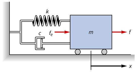
nssm = NonlinearStateSpaceModel[IconizedObject[«eqns»] /. IconizedObject[«pars»], {x[t], v[t]}, {f[t], Subscript[f, e][t]}, {x[t], v[t]}, t]小车对干扰力 fe 的开环响应没有调节,需要约40秒才能稳定下来:
OutputResponse[nssm, {0, 0.1 UnitStep[t]}, {t, 0, 60}];
Plot[%, {t, 0, 60}, PlotLegends -> {x, v}, PlotRange -> All]sspec = <|"InputModel" -> nssm, "FeedbackInputs" -> 1|>;wts = {DiagonalMatrix[{10, 1}], {{0.1}}};
τ = 0.4;dlqr = DiscreteLQRegulatorGains[sspec, wts, τ, "Data"]dcsys = dlqr["DiscreteTimeClosedLoopSystem"]or = OutputResponse[{dcsys, {0, 0.1}}, Table[{0, 0}, 20]];
ListStepPlot[%, DataRange -> {0, 19 τ}, PlotRange -> All, PlotLegends -> {x, v}]cm = dlqr["DiscreteTimeControllerModel"]OutputResponse[cm, Join[Table[{0}, 20], or]];
ListStepPlot[%, DataRange -> {0, 19 τ}, PlotRange -> All]
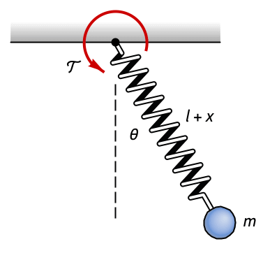
pend = NonlinearStateSpaceModel[IconizedObject[«eqns»] /. IconizedObject[«pars»], {x[t], x'[t], θ[t], θ'[t]}, 𝒯[t], {x[t], θ[t]}, t]OutputResponse[{pend, {0.1, 0, 0.2, 0}}, {0, 0}, {t, 0, 10}];
Plot[%, {t, 0, 10}, PlotRange -> All, PlotLegends -> {x, θ}]sspec = <|"InputModel" -> pend, "MeasuredOutputs" -> 2|>;wts = {DiagonalMatrix[{1, 1, 1, 1}], {{1}}};
τ = 0.5;dlqr = DiscreteLQRegulatorGains[sspec, wts, τ, "Data"]dcsys = dlqr["DiscreteTimeClosedLoopSystem"]sr = StateResponse[{dcsys, {0.1, 0, 0.2, 0}}, Table[{0, 0}, 60]];
ListStepPlot[{%[[1]], %[[3]]}, DataRange -> {0, 59 τ}, IconizedObject[«plotOpts»]]ControllableModelQ[StateSpaceModel[pend]]cm = dlqr["DiscreteTimeControllerModel"]OutputResponse[cm, Join[Table[{0, 0}, 60], sr]];
ListStepPlot[%, DataRange -> {0, 59 τ}, PlotRange -> All]poles = Table[Eigenvalues@First@Normal[sys], {sys, {dlqr["DiscreteTimeDesignModel"], StateSpaceModel[dcsys]}}];
Table[ListPlot[ReIm[{#}]& /@ poles[[i]], IconizedObject[«plotOpts»]], {i, 2}]
pend = NonlinearStateSpaceModel[IconizedObject[«eqns»] /. IconizedObject[«pars»], {θ[t], α[t], θ'[t], α'[t]}, Subscript[v, m][t], {θ[t], α[t]}, t]//Chop//FullSimplifyOutputResponse[{pend, {0.3, 0.2}}, 0, {t, 0, 300}];
Plot[%, {t, 0, 100}, PlotRange -> All, PlotLegends -> {θ, α}]wts = {DiagonalMatrix[{10^2, 10^4, 10, 10}], {{1}}};
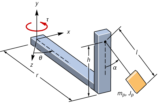
τ = 0.1;dlqr = DiscreteLQRegulatorGains[pend, wts, τ, "Data"]dcsys = dlqr["DiscreteTimeClosedLoopSystem"]sr = StateResponse[{dcsys, {0.1, 0.2}}, Table[0, 150 ]];
ListStepPlot[%[[{1, 2}]], DataRange -> {0, 149 τ}, IconizedObject[«plotOpts»]]dcm = dlqr["DiscreteTimeControllerModel"]OutputResponse[dcm, Join[{Table[0, 150 ]}, sr]];
ListStepPlot[%, DataRange -> {0, 149 τ}, PlotRange -> All]
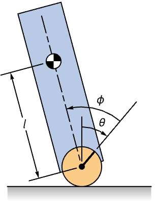
bbot = NonlinearStateSpaceModel[IconizedObject[«eqns»] /. IconizedObject[«pars»], {θ[t], ϕ[t], θ'[t], ϕ'[t]}, {Subscript[𝒯, 1][t], Subscript[𝒯, 2][t]}, {θ[t], ϕ[t]}, t]//Chop//Simplifyor = OutputResponse[{bbot, {0, 0.15, 0, 0}}, {0, 0}, {t, 0, 10}];Table[Plot[ℴ𝓇[[1]], {t, 0, 10}, IconizedObject[«plotOpts»]], {ℴ𝓇, ({or, {θ, ϕ}})}]wts = {10(| | | | |
| - | - | - | - |
| 5 | 0 | 0 | 0 |
| 0 | 5 | 0 | 0 |
| 0 | 0 | 1 | 0 |
| 0 | 0 | 0 | 1 |), 0.1(| | |
| - | - |
| 1 | 0 |
| 0 | 1 |)};
τ = 0.1;dlqr = DiscreteLQRegulatorGains[bbot, wts, τ, "Data"]dcsys = dlqr["DiscreteTimeClosedLoopSystem"]//Simplifysr = StateResponse[{dcsys, {0, 0.15, 0, 0}}, Table[{0, 0}, 60]];
ListStepPlot[{%[[1]], %[[2]]}, DataRange -> {0, 59 τ}, IconizedObject[«plotOpts»]]cm = dlqr["DiscreteTimeControllerModel"]//SimplifyOutputResponse[cm, Join[Table[{0, 0}, 60], sr]];
ListStepPlot[%, DataRange -> {0, 59 τ}, IconizedObject[«plotOpts»]]
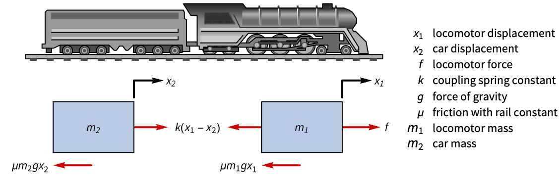
train = StateSpaceModel[IconizedObject[«eqns»] /. IconizedObject[«pars»], {Subscript[x, 1][t], Subscript[x, 2][t], Subscript[x, 1]'[t], Subscript[x, 2]'[t]}, f[t], {Subscript[x, 1][t], Subscript[x, 2][t]}, t, IconizedObject[«labels»]]OutputResponse[{train, {0.1, 0, 0, 0}}, 0, {t, 0, 100}];
Plot[%, {t, 0, 30}, PlotRange -> All, PlotLegends -> {Subscript[x, 1], Subscript[x, 2]}]Eigenvalues[First@Normal@train]//ChoptSig = Table[Splice[ConstantArray[i, 40]], {i, {2, 5, 9}}];
tSigPlot = ListStepPlot[%, IconizedObject[«plotOpts»]]sspec = <|"InputModel" -> train, "TrackedOutputs" -> 1|>;wts = {DiagonalMatrix[{1, 1, 1, 1, 1}], {{0.1}}};
τ = 0.2;dlqr = DiscreteLQRegulatorGains[sspec, wts, τ, "Data"]dcsys = dlqr["DiscreteTimeClosedLoopSystem"]sr = StateResponse[dcsys, tSig];Show[tSigPlot, ListStepPlot[Take[sr, 2], PlotLegends -> {Subscript[x, 1], Subscript[x, 2]}]]ListStepPlot[sr[[{3, 4}]], PlotLegends -> {Derivative[1][Subscript[x, 1]], Derivative[1][Subscript[x, 2]]}]dcm = dlqr["DiscreteTimeControllerModel"]cinps = Join[{tSig}, sr[[1 ;; 1]], sr[[1 ;; 4]]];ListStepPlot[OutputResponse[dcm, cinps]]航空航天系统 (3)
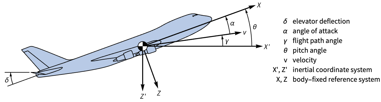
ssm = StateSpaceModel[IconizedObject[«eqns»], IconizedObject[«states»], δ[t], θ[t], t, IconizedObject[«labels»]]OutputResponse[{ssm, {0, 0, 0}}, UnitStep[t], {t, 0, 10}];
Plot[%, {t, 0, 10}, PlotRange -> All]PoleZeroPlot[ssm]wts = {DiagonalMatrix[{10, 10, 100}], {{0.1}}};
τ = 0.5;dlqr = DiscreteLQRegulatorGains[ssm, wts, τ, "Data"]dcsys = dlqr["DiscreteTimeClosedLoopSystem"]PoleZeroPlot[dcsys]sr = StateResponse[dcsys, Table[1, 30]];
ListStepPlot[sr[[3]], DataRange -> {0, 29 τ}, IconizedObject[«plotOpts»]]cm = dlqr["DiscreteTimeControllerModel"]OutputResponse[cm, Join[{Table[1, 30]}, sr]];
ListStepPlot[%, DataRange -> {0, 29 τ}, IconizedObject[«plotOpts»]]
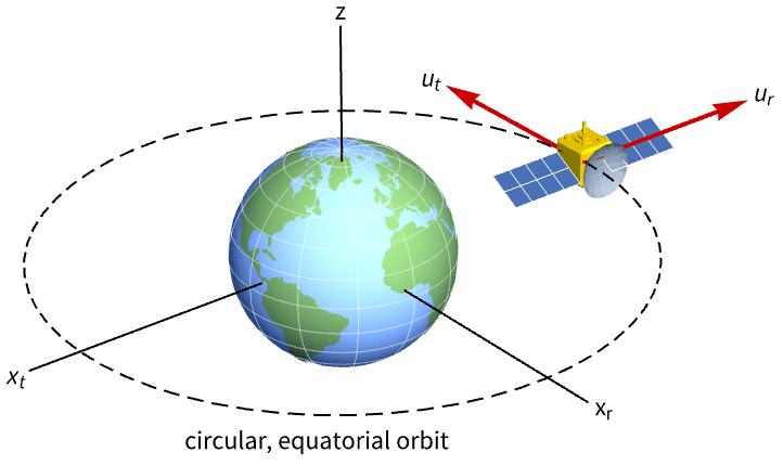
sat = StateSpaceModel[IconizedObject[«abc»], IconizedObject[«labels»]] /. ω -> 0.0011OutputResponse[{sat, {0, -1, 0, 1}}, {0, 0}, {t, 0, 10800}];
Plot[%, {t, 0, 10800}, PlotRange -> All, PlotLegends -> {Subscript[x, r], Subscript[x, t]}]如果切向推进器发生故障,轨道是可控的,但如果径向推进器发生故障,则轨道不可控:
Table[ControllableModelQ[SystemsModelExtract[sat, i]], {i, 2}]sspec = <|"InputModel" -> sat, "FeedbackInputs" -> 2|>;wts = {DiagonalMatrix[{1, 100, 1, 1}], {{1}}};
τ = 0.5;dlqr = DiscreteLQRegulatorGains[sspec, wts, τ, "Data"]dcsys = dlqr["DiscreteTimeClosedLoopSystem"]sr = StateResponse[{dcsys, {0, -1, 0, 1}}, Table[{0, 0}, 5400]];
ListStepPlot[sr[[{1, 3}]], DataRange -> {0, 5399 τ}, IconizedObject[«plotOpts»]]cm = dlqr["DiscreteTimeControllerModel"]OutputResponse[cm, Join[{Table[0, 5400]}, sr]];
ListStepPlot[%, DataRange -> {0, 5399 τ}, IconizedObject[«plotOpts»]]
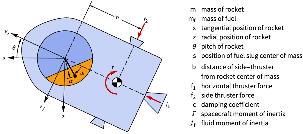
assm = AffineStateSpaceModel[IconizedObject[«eqns»] /. IconizedObject[«pars»], IconizedObject[«states»], {𝓇[t], Subscript[𝒻, 1][t], Subscript[𝒻, 2][t]}, {θ[t], ψ[t], ω[t], γ[t]}, t]OutputResponse[{assm, {0, 0.25, 0, 0, 0, -1}}, {0, 0, 0}, {t, 0, 60}];
Table[Plot[%[[i]], {t, 0, 60}, IconizedObject[«plotOpts»]], {i, 2}]ssm = StateSpaceModel[assm];
cm = ControllabilityMatrix[ssm];{MatrixRank[cm], SystemsModelOrder[ssm]}notC = Cases[Subsets[Range[8], {2}], _ ? (ControllableModelQ[SystemsModelDelete[ssm, None, None, #]]&)]Grid[Table[Part[IconizedObject[«states»], i], {i, notC}], IconizedObject[«gridOpts»]]assmDesign = SystemsModelDelete[assm, None, None, notC[[3]]]wts = {DiagonalMatrix[{10^7, 10^6, 1, 10^5, 10^5, 10^4}], DiagonalMatrix[{0.75, 1, 0.5}]};
τ = 0.01;dlqr = DiscreteLQRegulatorGains[assmDesign, wts, τ, "Data"]dcsys = dlqr[{"DiscreteTimeClosedLoopSystem"}]//Simplify//Chop[#, 10^-5]&sr = StateResponse[{dcsys, {0, 0.25, 0, 0, -1, 0}}, Table[{0, 0, 0}, 2000]];
Table[ListStepPlot[%[[i]], DataRange -> {0, 1999 τ}, IconizedObject[«plotOpts»]], {i, 2}]dcm = dlqr["DiscreteTimeControllerModel"]OutputResponse[dcm, Join[Table[{0, 0, 0}, 2000], sr]];
ListStepPlot[%, DataRange -> {0, 1999 τ}, IconizedObject[«plotOpts»]]生物系统 (1)
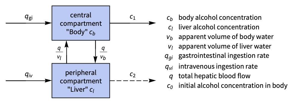
nssm = NonlinearStateSpaceModel[IconizedObject[«eqns»], {Subscript[c, b][t], Subscript[c, l][t]}, {Subscript[q, gi][t], Subscript[q, iv][t]}, Subscript[c, b][t], t] /. IconizedObject[«pars»]使用 StateSpaceModel 线性化系统:
ssm = N@StateSpaceModel[nssm, IconizedObject[«labels»]]StateResponse[{ssm, {12, 3}}, {0, 0}, {t, 0, 200}];
Table[Plot[𝓈𝓇[[1]], {t, 0, 200}, IconizedObject[«plotOpts»]], {𝓈𝓇, ({%, {Subscript[c, b], Subscript[c, l]}})}]wts = {DiagonalMatrix[{10000, 1}], DiagonalMatrix[{10^2, 10^4}]};
τ = 0.5;dlqr = DiscreteLQRegulatorGains[ssm, wts, τ, "Data"]dcsys = dlqr["DiscreteTimeClosedLoopSystem"]//Simplifysr = StateResponse[{dcsys, {12, 3}}, ConstantArray[{0, 0}, 300]];
Table[ListStepPlot[𝓈𝓇[[1]], IconizedObject[«plotOpts»]], {𝓈𝓇, ({%, {Subscript[c, b], Subscript[c, l]}})}]cm = dlqr["DiscreteTimeControllerModel"]OutputResponse[cm, Join[Table[{0, 0}, 300], sr]];
ListStepPlot[%, DataRange -> {0, 299 τ}, IconizedObject[«plotOpts»]]化学系统 (1)
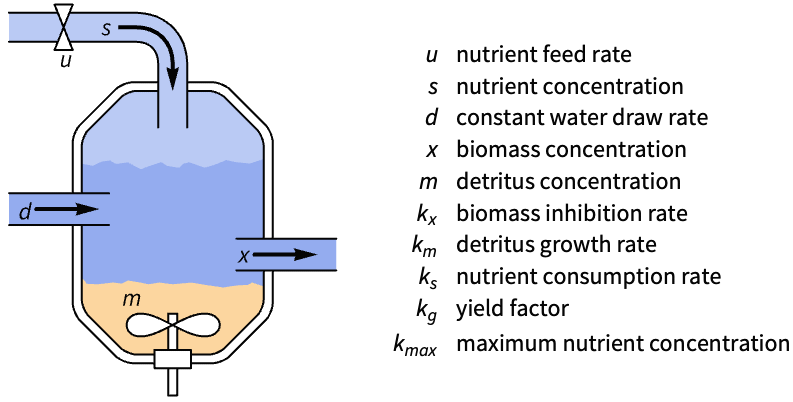
nssm = NonlinearStateSpaceModel[IconizedObject[«eqns»], {{x[t], Subscript[x, 0]}, {s[t], Subscript[s, 0]}, {m[t], Subscript[m, 0]}}, u[t], x[t], t] /. IconizedObject[«pars»]StateResponse[{nssm, {0.75, 0.01, 2}}, 0, {t, 0, 60}];
Plot[%, {t, 0, 60}, PlotRange -> All, PlotLegends -> {x, s, m}]sspec = <|"InputModel" -> nssm, "TrackedOutputs" -> 1|>;wts = {DiagonalMatrix[{10, 1, 1, 10^2}], {{300}}};
τ = 0.2;dlqr = DiscreteLQRegulatorGains[sspec, wts, τ, "Data"]dcsys = dlqr["DiscreteTimeClosedLoopSystem"]Subscript[x, ref] = 1.25;sr = StateResponse[{dcsys, {0.75, 0, 2}}, Table[Subscript[x, ref], 300]];ListStepPlot[sr[[1]], IconizedObject[«plotOpts»]]cm = dlqr["DiscreteTimeControllerModel"]cinps = Join[{Table[Subscript[x, ref], 300], sr[[1]]}, sr[[1 ;; 3]]];
ListStepPlot[OutputResponse[cm, cinps], PlotRange -> All]电气系统 (1)
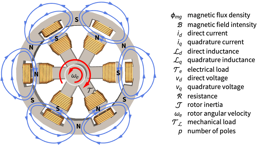
pmsm = NonlinearStateSpaceModel[IconizedObject[«eqns»] /. IconizedObject[«pars»], {Subscript[i, d][t], Subscript[i, q][t], Subscript[ω, e][t]}, {Subscript[v, d][t], Subscript[v, q][t], Subscript[𝒯, ℒ][t]}, Subscript[ω, e][t], t]//SimplifyOutputResponse[pmsm, {0, 0, UnitStep[t - 1]}, {t, 0, 1500}];
Plot[%, {t, 0, 1500}, PlotRange -> All]sspec = <|"InputModel" -> pmsm, "FeedbackInputs" -> {1, 2}|>;指定采样周期和一组控制权重,以实现最大 24 伏的控制力度:
τ = (1/60.0);
wts = {DiagonalMatrix[{1, 1, 1000}], DiagonalMatrix[{(1/24^2), (1/24^2)}]};dlqr = DiscreteLQRegulatorGains[sspec, wts, τ, "Data"]dcsys = dlqr["DiscreteTimeClosedLoopSystem"]//Chopsr = StateResponse[dcsys, Table[{0, 0, 1}, 1000]];
ListStepPlot[sr[[3]], DataRange -> {0, 999 τ}, PlotRange -> All]cm = dlqr["DiscreteTimeControllerModel"]OutputResponse[cm, Join[Table[{0, 0}, 1000], sr]];
ListStepPlot[%, DataRange -> {0, 999 τ}, IconizedObject[«plotOpts»]]船舶系统 (1)
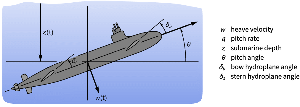
submarine = StateSpaceModel[IconizedObject[«abcd»], IconizedObject[«labels»]]如果没有控制器,潜艇的俯仰和深度对于以下状态的干扰是不稳定的:
OutputResponse[{submarine, {1, 0, 0.5, 0.2}}, {0, 0}, {t, 0, 20}];
Table[Plot[ℴ𝓇[[1]], {t, 0, 20}, IconizedObject[«plotOpts»]], {ℴ𝓇, ({%, {𝓏, θ}})}]sspec = <|"InputModel" -> submarine, "TrackedOutputs" -> {1, 2}|>;wts = {DiagonalMatrix[{5, 5, 10, 10, 10^3, 10^3}], 10^3IdentityMatrix[2]};
τ = 0.2;dlqr = DiscreteLQRegulatorGains[sspec, wts, τ, "Data"]dcsys = dlqr["DiscreteTimeClosedLoopSystem"]sr = StateResponse[dcsys, Table[{-10, 0}, 750]];
Table[ListStepPlot[𝓈𝓇[[1]], IconizedObject[«plotOpts»]], {𝓈𝓇, ({sr[[3 ;; 4]], {𝓏, θ}})}]cm = dlqr["DiscreteTimeControllerModel"]cinps = Join[Table[{-10, 0}, 750], sr[[{3, 4, 1, 2, 3, 4}]]];ListStepPlot[OutputResponse[cm, cinps], IconizedObject[«plotOpts»]]属性和关系 (5)
DiscreteLQRegulatorGains 计算为仿真离散时间系统的增益:
ssm = StateSpaceModel[{a = (| | |
| - | --- |
| 0 | 1 |
| 0 | -10 |), b = (| |
| - |
| 0 |
| 1 |), c = (1 0)}]{{q, r}, τ} = {{(| | |
| -- | - |
| 10 | 0 |
| 0 | 0 |), (1)}, 0.1};ssmd = ToDiscreteTimeModel[ssm, τ, Method -> "ZeroOrderHold"]ϕ = Subsuperscript[∫, 0, τ]MatrixExp[a t].q.MatrixExp[a t]ⅆtρ = Subsuperscript[∫, 0, τ](r + (Subsuperscript[∫, 0, t]MatrixExp[a η].bⅆη).q.Subsuperscript[∫, 0, t]MatrixExp[a η].bⅆη)ⅆtψ = Subsuperscript[∫, 0, τ]MatrixExp[a t].q.(Subsuperscript[∫, 0, t]MatrixExp[a η].bⅆη) ⅆtLQRegulatorGains[ssmd, {ϕ, ρ, ψ}]DiscreteLQRegulatorGains 给出相同的结果:
DiscreteLQRegulatorGains[ssm, {q, r}, τ]eqns = {Derivative[1][Subscript[x, 1]][t] == Subscript[x, 2][t], u[t] == -2 Subscript[x, 1][t] + Subscript[x, 2][t] + Derivative[1][Subscript[x, 2]][t]};
states = {Subscript[x, 1][t], Subscript[x, 2][t]};ssm = StateSpaceModel[eqns, states, u[t], Subscript[x, 1][t], t]τ = 0.4;
cd = DiscreteLQRegulatorGains[ssm, {(| | |
| - | - |
| 1 | 0 |
| 0 | 1 |), {{1}}}, τ, "Data"]dcsys = cd["DiscreteTimeClosedLoopSystem"]sr = StateResponse[{dcsys, {1, -1}}, Table[0, 10 / τ]];
p = ListStepPlot[%, IconizedObject[«plotOpts»]]fb = WhenEvent@@{Mod[t, τ] == 0, u[t] -> First[-cd["FeedbackGains"].states]}ceqns = Join[eqns, {Subscript[x, 1][0] == 1, Subscript[x, 2][0] == -1, u[0] == 0}, {fb}]NDSolve[ceqns, Join[states, {u[t]}], {t, 0, 7}, DiscreteVariables -> u[t]];
csols = First[states /. %]Legended[Show[Plot[csols, {t, 0, 7}, IconizedObject[«plotOpts»]], p], IconizedObject[«lineLegend»]]τ = {0.4, 0.1, 0.025};{dcsys, κ} = Table[DiscreteLQRegulatorGains[IconizedObject[«ssm»], IconizedObject[«wts»], i, IconizedObject[«props»]], {i, τ}];Grid[{dcsys, κ}, IconizedObject[«gridOpts»]]sr = Table[StateResponse[{dcsys[[i]], {1, -1}}, Table[0, 8 / τ[[i]]]], {i, 3}];
p = Table[ListStepPlot[sr[[i, k]], DataRange -> {0, 8}, IconizedObject[«plotOpts»]], {i, 3}, {k, 2}]sols = Table[NDSolve[{IconizedObject[«ssmEqns»], Subscript[x, 1][0] == 1, Subscript[x, 2][0] == -1, u[0] == 0, WhenEvent[Mod[t, τ[[i]]] == 0, u[t] -> -First[κ[[i]].IconizedObject[«states»]]]}, Join[IconizedObject[«states»], {u[t]}], {t, 0, 8}, DiscreteVariables -> u[t]], {i, 3}];Shallow[xSols = Table[First[IconizedObject[«states»] /. %[[i]]], {i, 3}]]Table[Legended[Show[Plot[Evaluate@xSols[[i, k]], {t, 0, 8}, IconizedObject[«plotOpts»]], p[[i, k]]], IconizedObject[«leg»]], {i, 3}, {k, 2}];
Grid[%, Spacings -> {2.5, 1}]τ = {0.4, 0.1, 0.025};Short[sr = IconizedObject[«sr»]]Short[sols = IconizedObject[«sols»]]dcm = Table[DiscreteLQRegulatorGains[IconizedObject[«ssm»], IconizedObject[«wts»], i, "DiscreteTimeControllerModel"], {i, τ}]ce = Table[OutputResponse[dcm[[i]], Join[{Table[0, 8 / τ[[i]]]}, sr[[i]]]], {i, 3}];
p = Table[ListStepPlot[ce[[i]], DataRange -> {0, 8}, IconizedObject[«plotOpts»]], {i, 3}]csols = Table[First[{u[t]} /. sols[[i]]], {i, 3}]Table[Legended[Show[Plot[csols[[i]], {t, 0, 8}, IconizedObject[«plotOpts»]], p[[i]]], IconizedObject[«leg»]], {i, 3}]缩短采样周期会导致闭环极点更接近单位圆,即更接近不稳定状态:
τ = {0.4, 0.1, 0.025};dcsys = Table[DiscreteLQRegulatorGains[IconizedObject[«ssm»], IconizedObject[«wts»], i, "DiscreteTimeClosedLoopSystem"], {i, τ}]Table[Eigenvalues@First@Normal[dcsys[[i]]], {i, 3}];
Grid[{{"τ = 0.4", "τ = 0.1", "τ = 0.025"}, %}, IconizedObject[«gridOpts»]]可能存在的问题 (1)
ssm = StateSpaceModel[{{{-3, 1}, {0, 2}}, {{1}, {0}}, {{1, 0}, {0, 1}}, {{0}, {0}}},
SamplingPeriod -> None, SystemsModelLabels -> None];DiscreteLQRegulatorGains[ssm, {(| | |
| - | -- |
| 1 | 0 |
| 0 | 1. |), (1)}, 1]Table[{λ, ControllableModelQ[{ssm, λ}]}, {λ, Eigenvalues[Normal[ssm][[1]]]}]相关指南
-
▪
- 使用状态空间模型进行设计 ▪
- 控制系统
文本
Wolfram Research (2010),DiscreteLQRegulatorGains,Wolfram 语言函数,https://reference.wolfram.com/language/ref/DiscreteLQRegulatorGains.html (更新于 2021 年).
CMS
Wolfram 语言. 2010. "DiscreteLQRegulatorGains." Wolfram 语言与系统参考资料中心. Wolfram Research. 最新版本 2021. https://reference.wolfram.com/language/ref/DiscreteLQRegulatorGains.html.
APA
Wolfram 语言. (2010). DiscreteLQRegulatorGains. Wolfram 语言与系统参考资料中心. 追溯自 https://reference.wolfram.com/language/ref/DiscreteLQRegulatorGains.html 年
BibTeX
@misc{reference.wolfram_2026_discretelqregulatorgains, author="Wolfram Research", title="{DiscreteLQRegulatorGains}", year="2021", howpublished="\url{https://reference.wolfram.com/language/ref/DiscreteLQRegulatorGains.html}", note=[Accessed: 12-September-2026]}
BibLaTeX
@online{reference.wolfram_2026_discretelqregulatorgains, organization={Wolfram Research}, title={DiscreteLQRegulatorGains}, year={2021}, url={https://reference.wolfram.com/language/ref/DiscreteLQRegulatorGains.html}, note=[Accessed: 12-September-2026]}