EvaluationMonitor

多くの数値計算およびプロット関数のオプションで，入力から派生した関数が数値的に評価される際に評価する式を与える．

詳細

オプション設定は通常EvaluationMonitor:>expr として与えられる．expr が即時に評価されるのを避けるために，->ではなく:>が使われる．
expr が評価されると，数値計算におけるすべての変数に現行の値が割り当てられる．実際はBlock[{var₁=val₁,…},expr]が使われる． »

例題

すべて開くすべて閉じる

例 (4)

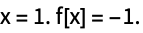
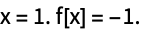
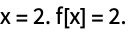
根を求めるのに使われたすべての関数評価を含む情報を出力する：

Wolfram Language code: FindRoot[x ^ 2 - 2, {x, 1}, EvaluationMonitor :> Print["x = ", x, " x^2 - 2 =", x ^ 2 - 2]]

評価を数える：

Wolfram Language code: Block[{c = 0}, {FindRoot[x ^ 2 - 2, {x, 1}, EvaluationMonitor :> c++], c}]

ReapとSowを使って評価データを収集する：

Wolfram Language code: {res, data} = Reap[FindRoot[x ^ 2 - 2, {x, 1}, EvaluationMonitor :> Sow[x - Sqrt[2]]]]

メソッドの超一次収束を示す：

Wolfram Language code: ListLogLogPlot[data[[1]]]

波動方程式の時間積分をモニターする：

Wolfram Language code:

Monitor[NDSolveValue[{D[u[t, x, y], {t, 2}] == Laplacian[u[t, x, y], {x, y}], u[0, x, y] == 0, Derivative[1, 0, 0][u][0, x, y] == 0, DirichletCondition[u[t, x, y] == If[t < 1, t, 1], x == 0]}, u, {x, y}∈RegionUnion[Rectangle[{0, 0}, {5, 1}], Disk[{5, 1 / 2}, 1 / 2]], {t, 0, 10}
	, EvaluationMonitor :> (monitor = Row[{"t = ", CForm[t]}])], monitor]

スコープ (5)

正弦Gordonの偏微分方程式を解く際の解の進行をモニターする：

Wolfram Language code:

Monitor[NDSolve[{Subscript[∂, t, t]u[t, x] == Subscript[∂, x, x]u[t, x] + Sin[u[t, x]] , u[0, x] == E^-x^2, u^(1, 0)[0, x] == 0, u[t, -10] == u[t, 10]}, u, {t, 0, 10}, {x, -10, 10}, EvaluationMonitor :> (sol = u[t, x]; time = t)], Plot[sol, {x, -10, 10}, PlotRange -> {0, 8}, PlotLabel -> time]]

数値的最小化の評価：

Wolfram Language code: {res, data} = Reap[FindMinimum[(x - 1) ^ 2 + 100(y - Sin[x]) ^ 2, {{x, -10}, {y, 1}}, EvaluationMonitor :> Sow[{x, y}]]]

Wolfram Language code: ListPlot[data[[1]]]

NIntegrateを使って数値積分を計算するための評価：

Wolfram Language code: {res, data} = Reap[NIntegrate[Sqrt[x(1 - x)], {x, 0, 1}, EvaluationMonitor :> Sow[x]]];

Wolfram Language code: res

評価位置対評価回数のプロットを示す：

Wolfram Language code: ListPlot[data[[1]]]

NDSolveと外挿法を使って微分方程式を解く際の評価：

Wolfram Language code:

{sol, evals} = Reap[NDSolve[{x''[t] + Sin[x[t]] == 0, x[0] == 1, x'[0] == 0}, x, {t, 0, 10}, EvaluationMonitor :> Sow[{t, x[t], x'[t]}], Method -> "Extrapolation"]];

プロットは，この方法ではすべての評価が解の曲線上にある訳ではないことを示している：

Wolfram Language code:

Show[Plot[Evaluate[First[{x[t], x'[t]} /. sol]], {t, 0, 10}], ListPlot[{evals[[1, All, {1, 2}]], evals[[1, All, {1, 3}]]}]]

曲面プロットのための評価数を数える：

Wolfram Language code: f[x_, y_] := E^x - Sin[x^3 - 3 y];

Wolfram Language code:

Block[{c = 0}, Plot3D[f[x, y], {x, -2, 2}, {y, -2, 2}, EvaluationMonitor :> c++, PlotLabel :> ToString[c] <> " evaluations"]]

記号導関数が使われているので，関数評価に使われる評価回数は少なくなる：

Wolfram Language code:

Block[{c = 0}, Plot3D[Evaluate[f[x, y]], {x, -2, 2}, {y, -2, 2}, EvaluationMonitor :> c++, PlotLabel :> ToString[c] <> " evaluations"]]

一般化と拡張 (2)

任意の式を評価する：

Wolfram Language code: Catch[FindMinimum[Exp[x] + 1 / x ^ 2, {x, 1}, EvaluationMonitor :> If[x ≤ 0, Throw["Negative x"]]]]

別の初期値を使うと計算が停止される：

Wolfram Language code: Catch[FindMinimum[Exp[x] + 1 / x ^ 2, {x, 10}, EvaluationMonitor :> If[x ≤ 0, Throw["Negative x"]]]]

数値的最小化を行う際に関数評価と導関数評価を区別する：

Wolfram Language code:

{sol, evaldata} = Reap[FindMinimum[(x - 1) ^ 2 + 100(y - x ^ 2) ^ 2, {{x, -1}, {y, 1}}, EvaluationMonitor :> Sow[{x, y}, 0], Gradient -> {"Symbolic", EvaluationMonitor :> Sow[{x, y}, 1]}, 
	Method -> {"Newton", "Hessian" -> {"Symbolic", EvaluationMonitor :> Sow[{x, y}, 2]}}], _, Rule];sol

関数，勾配，ヘッセン方程式をそれぞれ青，赤，黄で示す：

Wolfram Language code:

colors = {Blue, Yellow, Red};
sizes = {PointSize[0.015], PointSize[0.03], PointSize[0.05]};ContourPlot[(x - 1) ^ 2 + 100(y - x ^ 2) ^ 2, {x, -1, 1}, {y, -1, 1}, Epilog -> Table[{colors[[i + 1]], sizes[[i + 1]], Map[Point, i /. evaldata]}, {i, 2, 0, -1}]]

アプリケーション (6)

順番を示すツールチップを用いてプロットのどの部分で評価が行われたかを示す：

Wolfram Language code:

f[x_] = Exp[-x ^ 2];
{plot, evals} = Reap[Block[{e = 0}, Plot[f[x], {x, -5, 5}, PlotRange -> All, EvaluationMonitor :> Sow[Tooltip[Point[{x, f[x]}], ++e]]]]];
Show[plot, Graphics[{Red, evals}]]

根を求めるために必要な評価数を初期値の関数として求める：

Wolfram Language code: evals[sv_ ? NumberQ] := Block[{c = 0}, FindRoot[Cos[x], {x, sv}, EvaluationMonitor :> c++];c]

Wolfram Language code: Plot[evals[sv], {sv, 0, π}]

極小値を求める各メソッドで必要な評価を比べる：

Wolfram Language code:

TableForm[Table[ Block[{e = 0}, {method, Norm[{x - 1, y - 1} /. FindMinimum[(x - 1) ^ 2 + 100(y - x ^ 2) ^ 2, {{x, -1}, {y, 1}}, Method -> method, EvaluationMonitor :> e++][[2]]], e}], {method, {Automatic, "LevenbergMarquardt", "Newton", "QuasiNewton", "Gradient"}}], TableHeadings -> {{}, {"Method", "Error", "Evaluations"}} ]

NDSolveの各ODE積分法に必要な評価数と時間を比較する：

Wolfram Language code:

evals[method_] := Block[{e = 0}, Timing[NDSolve[{x''[t] + x[t] == 0, x[0] == 1, x'[0] == 0}, x, {t, 0, 100π}, MaxSteps -> Infinity, Method -> method, EvaluationMonitor :> e++];e]]

Wolfram Language code: methods = {Automatic, "Adams", "BDF", "ExplicitRungeKutta", "ImplicitRungeKutta", "Extrapolation"};

Wolfram Language code:

TableForm[Table[Join[{method}, evals[method]], {method, methods}], TableHeadings -> {{}, {"Method", "Timing", "Evaluations"}}]

NDSolveのPrecisionGoalとAccuracyGoalの関数としてのステップと評価：

Wolfram Language code:

se[method_][g_] := Block[{s = 0, e = 0}, NDSolve[{x''[t] + x'[t] / 10 + x[t] / (1 + x[t] ^ 2) == Sin[t], x[0] == 1, x'[0] == 0}, x, {t, 0, 100}, PrecisionGoal -> g, AccuracyGoal -> g, WorkingPrecision -> If[g > 8, 2g, MachinePrecision], StepMonitor :> s++, EvaluationMonitor :> e++, MaxSteps -> Infinity, Method -> method];{s, e}]

固定次数の明示的ルンゲ・クッタ(Runge–Kutta)法を使う：

Wolfram Language code: erk = Table[Flatten[{g, se[{"ExplicitRungeKutta", "DifferenceOrder" -> 8}][g]}], {g, 0, 20, 2}]

適応的順の外挿法を使う：

Wolfram Language code: ext = Table[Flatten[{g, se["Extrapolation"][g]}], {g, 0, 20, 2}]

2つのメソッドを比較する．12を超えるゴールでは，明らかに適応的順が優れている：

Wolfram Language code:

ListLogPlot[{erk[[All, {1, 2}]], erk[[All, {1, 3}]], ext[[All, {1, 2}]], ext[[All, {1, 3}]]}, PlotStyle -> {Purple, Red, Orange, Blue}]

非線形フィットのためのパラメータ空間における評価：

Wolfram Language code:

data = {{0.18, -0.13}, {0.84, -0.06}, {0.05, 0.88}, {0.24, -0.63}, {0.67, 0.93}, {0.05, 0.88}, {0.65, 0.92}, {0.01, 0.99}, {0.17, -0.04}, {0.23, -0.55}};

Wolfram Language code: model[{w_, p_}] = Exp[-0.1 x] Sin[w x + p];

Wolfram Language code: {fit, {evals}} = Reap[FindFit[data, model[{w, p}], {w, p}, x, EvaluationMonitor :> Sow[{w, p}]]]

平方和の等高線プロット上の評価点：

Wolfram Language code:

residual = Map[Function[{x}, Evaluate[model[{w, p}]]], data[[All, 1]]] - data[[All, 2]];
ContourPlot[Evaluate[residual.residual], {w, 0, 10}, {p, 0, 2 π}, Epilog -> {Red, Point[evals]}]

より適切な初期値を使う：

Wolfram Language code: {bfit, {bevals}} = Reap[FindFit[data, model[{w, p}], {{w, 4}, {p, 4}}, x, EvaluationMonitor :> Sow[{w, p}]]]

Wolfram Language code:

ContourPlot[Evaluate[residual.residual], {w, 0, 10}, {p, 0, 2 π}, Epilog -> {{Red, Point[evals]}, {Green, Point[bevals]}}]

2つのフィットをデータと比べる：

Wolfram Language code: Show[Plot[Evaluate[model[{w, p}] /. {fit, bfit}], {x, 0, 1}, PlotStyle -> {{Red}, {Green}}], ListPlot[data]]

特性と関係 (1)

EvaluationMonitorによる評価はBlockのように調べられる：

Wolfram Language code: f[x_] := x ^ 2 - 2;

Wolfram Language code: FindRoot[f[x], {x, 1, 2}, EvaluationMonitor :> Print["x = ", x, " f[x] = ", f[x]]]

これは実質的にBlockを変数の数値の割当てとともに使うのに等しい：

Wolfram Language code: ff[xx_ ? NumberQ] := Block[{x = xx}, Print["x = ", x, " f[x] = ", f[x]];f[x]]

Wolfram Language code: FindRoot[ff[x], {x, 1, 2}]

Top

その他のラーニングリソース

テクニカルサポート

データサイエンス，金融，ビジネス

工学

科学とテクノロジー

教育のためのテクノロジー

教育イニシアチブ

使い始める

Grow Your Skills

Wolframと繋がる

大人用の教育プログラム

若者のための教育プログラム

読む

EvaluationMonitor

詳細

例題

例 (4)

スコープ (5)

一般化と拡張 (2)

アプリケーション (6)

特性と関係 (1)

テキスト

CMS

APA

BibTeX

BibLaTeX

EvaluationMonitor

詳細

例題

例 (4)

スコープ (5)

一般化と拡張 (2)

アプリケーション (6)

特性と関係 (1)

関連項目

テクニカルノート

関連するガイド

関連するワークフロー

履歴

テキスト

CMS

APA

BibTeX

BibLaTeX