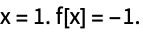
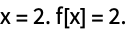
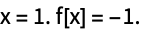
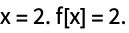
是一个选项,用于各种数值计算和绘图功能,每当对从输入导出的函数进行数值计算时,就给出一个表达式进行计算.

EvaluationMonitor
是一个选项,用于各种数值计算和绘图功能,每当对从输入导出的函数进行数值计算时,就给出一个表达式进行计算.
范例
打开所有单元 关闭所有单元基本范例 (4)

FindRoot[x ^ 2 - 2, {x, 1}, EvaluationMonitor :> Print["x = ", x, " x^2 - 2 =", x ^ 2 - 2]]Block[{c = 0}, {FindRoot[x ^ 2 - 2, {x, 1}, EvaluationMonitor :> c++], c}]{res, data} = Reap[FindRoot[x ^ 2 - 2, {x, 1}, EvaluationMonitor :> Sow[x - Sqrt[2]]]]ListLogLogPlot[data[[1]]]Monitor[NDSolveValue[{D[u[t, x, y], {t, 2}] == Laplacian[u[t, x, y], {x, y}], u[0, x, y] == 0, Derivative[1, 0, 0][u][0, x, y] == 0, DirichletCondition[u[t, x, y] == If[t < 1, t, 1], x == 0]}, u, {x, y}∈RegionUnion[Rectangle[{0, 0}, {5, 1}], Disk[{5, 1 / 2}, 1 / 2]], {t, 0, 10}
, EvaluationMonitor :> (monitor = Row[{"t = ", CForm[t]}])], monitor]范围 (5)
Monitor[NDSolve[{Subscript[∂, t, t]u[t, x] == Subscript[∂, x, x]u[t, x] + Sin[u[t, x]] , u[0, x] == E^-x^2, u^(1, 0)[0, x] == 0, u[t, -10] == u[t, 10]}, u, {t, 0, 10}, {x, -10, 10}, EvaluationMonitor :> (sol = u[t, x]; time = t)], Plot[sol, {x, -10, 10}, PlotRange -> {0, 8}, PlotLabel -> time]]{res, data} = Reap[FindMinimum[(x - 1) ^ 2 + 100(y - Sin[x]) ^ 2, {{x, -10}, {y, 1}}, EvaluationMonitor :> Sow[{x, y}]]]ListPlot[data[[1]]]这些计算用于利用 NIntegrate 计算一个数值积分:
{res, data} = Reap[NIntegrate[Sqrt[x(1 - x)], {x, 0, 1}, EvaluationMonitor :> Sow[x]]];resListPlot[data[[1]]]用使用外插法的 NDSolve 进行求解一个微分方程的计算:
{sol, evals} = Reap[NDSolve[{x''[t] + Sin[x[t]] == 0, x[0] == 1, x'[0] == 0}, x, {t, 0, 10}, EvaluationMonitor :> Sow[{t, x[t], x'[t]}], Method -> "Extrapolation"]];Show[Plot[Evaluate[First[{x[t], x'[t]} /. sol]], {t, 0, 10}], ListPlot[{evals[[1, All, {1, 2}]], evals[[1, All, {1, 3}]]}]]f[x_, y_] := E^x - Sin[x^3 - 3 y];Block[{c = 0}, Plot3D[f[x, y], {x, -2, 2}, {y, -2, 2}, EvaluationMonitor :> c++, PlotLabel :> ToString[c] <> " evaluations"]]Block[{c = 0}, Plot3D[Evaluate[f[x, y]], {x, -2, 2}, {y, -2, 2}, EvaluationMonitor :> c++, PlotLabel :> ToString[c] <> " evaluations"]]推广和延伸 (2)
Catch[FindMinimum[Exp[x] + 1 / x ^ 2, {x, 1}, EvaluationMonitor :> If[x ≤ 0, Throw["Negative x"]]]]Catch[FindMinimum[Exp[x] + 1 / x ^ 2, {x, 10}, EvaluationMonitor :> If[x ≤ 0, Throw["Negative x"]]]]{sol, evaldata} = Reap[FindMinimum[(x - 1) ^ 2 + 100(y - x ^ 2) ^ 2, {{x, -1}, {y, 1}}, EvaluationMonitor :> Sow[{x, y}, 0], Gradient -> {"Symbolic", EvaluationMonitor :> Sow[{x, y}, 1]},
Method -> {"Newton", "Hessian" -> {"Symbolic", EvaluationMonitor :> Sow[{x, y}, 2]}}], _, Rule];solcolors = {Blue, Yellow, Red};
sizes = {PointSize[0.015], PointSize[0.03], PointSize[0.05]};ContourPlot[(x - 1) ^ 2 + 100(y - x ^ 2) ^ 2, {x, -1, 1}, {y, -1, 1}, Epilog -> Table[{colors[[i + 1]], sizes[[i + 1]], Map[Point, i /. evaldata]}, {i, 2, 0, -1}]]应用 (6)
f[x_] = Exp[-x ^ 2];
{plot, evals} = Reap[Block[{e = 0}, Plot[f[x], {x, -5, 5}, PlotRange -> All, EvaluationMonitor :> Sow[Tooltip[Point[{x, f[x]}], ++e]]]]];
Show[plot, Graphics[{Red, evals}]]evals[sv_ ? NumberQ] := Block[{c = 0}, FindRoot[Cos[x], {x, sv}, EvaluationMonitor :> c++];c]Plot[evals[sv], {sv, 0, π}]TableForm[Table[ Block[{e = 0}, {method, Norm[{x - 1, y - 1} /. FindMinimum[(x - 1) ^ 2 + 100(y - x ^ 2) ^ 2, {{x, -1}, {y, 1}}, Method -> method, EvaluationMonitor :> e++][[2]]], e}], {method, {Automatic, "LevenbergMarquardt", "Newton", "QuasiNewton", "Gradient"}}], TableHeadings -> {{}, {"Method", "Error", "Evaluations"}} ]比较在 NDSolve 中不同的常微分方程积分法所需的计算和时序:
evals[method_] := Block[{e = 0}, Timing[NDSolve[{x''[t] + x[t] == 0, x[0] == 1, x'[0] == 0}, x, {t, 0, 100π}, MaxSteps -> Infinity, Method -> method, EvaluationMonitor :> e++];e]]methods = {Automatic, "Adams", "BDF", "ExplicitRungeKutta", "ImplicitRungeKutta", "Extrapolation"};TableForm[Table[Join[{method}, evals[method]], {method, methods}], TableHeadings -> {{}, {"Method", "Timing", "Evaluations"}}]作为在 NDSolve 中 PrecisionGoal 和 AccuracyGoal 函数的步骤和计算:

se[method_][g_] := Block[{s = 0, e = 0}, NDSolve[{x''[t] + x'[t] / 10 + x[t] / (1 + x[t] ^ 2) == Sin[t], x[0] == 1, x'[0] == 0}, x, {t, 0, 100}, PrecisionGoal -> g, AccuracyGoal -> g, WorkingPrecision -> If[g > 8, 2g, MachinePrecision], StepMonitor :> s++, EvaluationMonitor :> e++, MaxSteps -> Infinity, Method -> method];{s, e}]erk = Table[Flatten[{g, se[{"ExplicitRungeKutta", "DifferenceOrder" -> 8}][g]}], {g, 0, 20, 2}]ext = Table[Flatten[{g, se["Extrapolation"][g]}], {g, 0, 20, 2}]比较两种方法. 超过目标 12 左右时,适应性顺序明显优越:
ListLogPlot[{erk[[All, {1, 2}]], erk[[All, {1, 3}]], ext[[All, {1, 2}]], ext[[All, {1, 3}]]}, PlotStyle -> {Purple, Red, Orange, Blue}]data = {{0.18, -0.13}, {0.84, -0.06}, {0.05, 0.88}, {0.24, -0.63}, {0.67, 0.93}, {0.05, 0.88}, {0.65, 0.92}, {0.01, 0.99}, {0.17, -0.04}, {0.23, -0.55}};model[{w_, p_}] = Exp[-0.1 x] Sin[w x + p];{fit, {evals}} = Reap[FindFit[data, model[{w, p}], {w, p}, x, EvaluationMonitor :> Sow[{w, p}]]]residual = Map[Function[{x}, Evaluate[model[{w, p}]]], data[[All, 1]]] - data[[All, 2]];
ContourPlot[Evaluate[residual.residual], {w, 0, 10}, {p, 0, 2 π}, Epilog -> {Red, Point[evals]}]{bfit, {bevals}} = Reap[FindFit[data, model[{w, p}], {{w, 4}, {p, 4}}, x, EvaluationMonitor :> Sow[{w, p}]]]ContourPlot[Evaluate[residual.residual], {w, 0, 10}, {p, 0, 2 π}, Epilog -> {{Red, Point[evals]}, {Green, Point[bevals]}}]Show[Plot[Evaluate[model[{w, p}] /. {fit, bfit}], {x, 0, 1}, PlotStyle -> {{Red}, {Green}}], ListPlot[data]]属性和关系 (1)
EvaluationMonitor 的计算范围同 Block 一样:
f[x_] := x ^ 2 - 2;FindRoot[f[x], {x, 1, 2}, EvaluationMonitor :> Print["x = ", x, " f[x] = ", f[x]]]它实际利用带有变量数值赋值的 Block:
ff[xx_ ? NumberQ] := Block[{x = xx}, Print["x = ", x, " f[x] = ", f[x]];f[x]]FindRoot[ff[x], {x, 1, 2}]技术笔记
-
▪
- 监控和选择算法
历史
2003年引入 (5.0) | 在以下年份被更新:2007 (6.0)
文本
Wolfram Research (2003),EvaluationMonitor,Wolfram 语言函数,https://reference.wolfram.com/language/ref/EvaluationMonitor.html (更新于 2007 年).
CMS
Wolfram 语言. 2003. "EvaluationMonitor." Wolfram 语言与系统参考资料中心. Wolfram Research. 最新版本 2007. https://reference.wolfram.com/language/ref/EvaluationMonitor.html.
APA
Wolfram 语言. (2003). EvaluationMonitor. Wolfram 语言与系统参考资料中心. 追溯自 https://reference.wolfram.com/language/ref/EvaluationMonitor.html 年
BibTeX
@misc{reference.wolfram_2026_evaluationmonitor, author="Wolfram Research", title="{EvaluationMonitor}", year="2007", howpublished="\url{https://reference.wolfram.com/language/ref/EvaluationMonitor.html}", note=[Accessed: 13-September-2026]}
BibLaTeX
@online{reference.wolfram_2026_evaluationmonitor, organization={Wolfram Research}, title={EvaluationMonitor}, year={2007}, url={https://reference.wolfram.com/language/ref/EvaluationMonitor.html}, note=[Accessed: 13-September-2026]}