RiccatiSolve[{a,b},{q,r}]
gives the matrix ![]() that is the stabilizing solution of the continuous algebraic Riccati equation
that is the stabilizing solution of the continuous algebraic Riccati equation ![]() .
.
RiccatiSolve[{a,b},{q,r,p}]
solves the equation ![]() .
.


RiccatiSolve
RiccatiSolve[{a,b},{q,r}]
gives the matrix ![]() that is the stabilizing solution of the continuous algebraic Riccati equation
that is the stabilizing solution of the continuous algebraic Riccati equation ![]() .
.
RiccatiSolve[{a,b},{q,r,p}]
solves the equation ![]() .
.
Details and Options

- In
![TemplateBox[{a}, ConjugateTranspose].x+x.a-x.b.TemplateBox[{r}, Inverse].TemplateBox[{b}, ConjugateTranspose].x+q=0 TemplateBox[{a}, ConjugateTranspose].x+x.a-x.b.TemplateBox[{r}, Inverse].TemplateBox[{b}, ConjugateTranspose].x+q=0](Files/RiccatiSolve.en/4.png) ,
,  denotes the conjugate transpose.
 - The equation
![TemplateBox[{a}, ConjugateTranspose].x+x.a-x.b.TemplateBox[{r}, Inverse].TemplateBox[{b}, ConjugateTranspose].x+q=0 TemplateBox[{a}, ConjugateTranspose].x+x.a-x.b.TemplateBox[{r}, Inverse].TemplateBox[{b}, ConjugateTranspose].x+q=0](Files/RiccatiSolve.en/6.png) has a unique, symmetric, positive semidefinite solution
has a unique, symmetric, positive semidefinite solution  if
if  is stabilizable,
  is detectable,
  , and
, and  . Consequently, all eigenvalues of the matrix
  are negative and the solution is stabilizing.
 - The solution is positive definite when
 is controllable and
  is observable.
 - RiccatiSolve supports a Method option, with the following possible settings:
-
Automatic automatically determined method "Eigensystem" based on eigen decomposition "GeneralizedEigensystem" based on generalized eigen decomposition "GeneralizedSchur" based on generalized Schur decomposition "InverseFree" a variant of "GeneralizedSchur" "MatrixSign" iterative method using the matrix sign function "Newton" iterative Newton method "Schur" based on Schur decomposition - All methods apply to approximate numeric matrices. "Eigensystem" also applies to exact matrices.
Examples
open all close allScope (3)
Options (7)
Method (7)
Automatic and "Eigensystem" methods can be used for exact systems:
As well as for inexact systems:
"Schur" method can be used for inexact systems:
"Newton" applies to inexact systems and may be more accurate than Automatic:
Compute the solution and absolute error:
Compare to the default method:
"Newton" takes suboptions "StartingMatrix", "MaxIterations", and "Tolerance":
The "Newton" method may not converge even if a stabilizing solution exists:
Compare with the Automatic method:
"MatrixSign" is typically used as an initial approximation for the "Newton" method:
Use xinit to initialize the "Newton" method:
"MatrixSign" takes suboptions "MaxIterations" and "Tolerance":
"GeneralizedSchur" and "GeneralizedEigensystem" applies when a is singular:
These two methods work for a singular a:
"InverseFree" can be used when r is ill-conditioned:
The matrix r has a high condition number:
Compare to the default method:
The absolute error is higher for the default method in this case:
Applications (3)
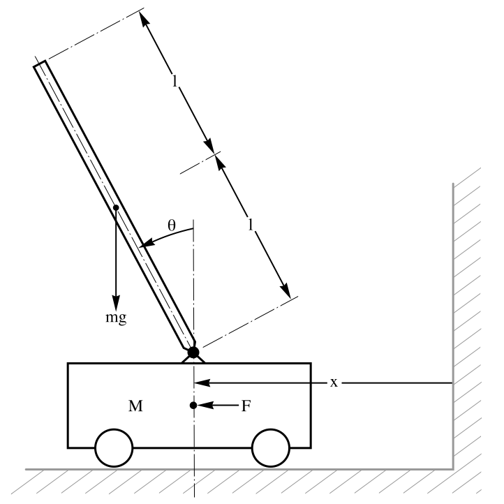
Compute the cost associated with an optimal trajectory for a linearized inverted pendulum:

Obtain the cost by numerical integration:
Track the "cost to go" at each instant along the optimal trajectory:
Compute an optimal state-feedback gain that places all closed-loop poles to the left of ![]() :
:
The closed-loop poles without any prescribed degree of stability:
Compute the minimum error covariance for a Kalman estimator:
Properties & Relations (8)
Find the optimal gains with cross-coupling matrix p:
An equivalent result can be found be incorporating p into the a and q matrices:
If {a,b} is controllable and {a,g} is observable, and q=Transpose[g].g, then the solution to the Riccati equation is positive definite:
The eigenvalues of the Hamiltonian matrix ![]() are pairs of the form {λ,-λ}:
are pairs of the form {λ,-λ}:
The ability to obtain a stabilizing solution depends on the Hamiltonian matrix:
The Hamiltonian matrix must satisfy the stability property:
As well as the complementarity property:
Find the eigenvalues of the feedback system with ![]() :
:
These are also the stable eigenvalues of the Hamiltonian matrix:
Compute optimal state feedback gains using RiccatiSolve:
Use LQRegulatorGains to compute the same result directly:
Compute optimal output feedback gains using RiccatiSolve:
LQOutputRegulatorGains gives the same result:
Compute optimal estimator gains using RiccatiSolve:
Use LQEstimatorGains to compute this result directly:
Related Guides
Text
Wolfram Research (2010), RiccatiSolve, Wolfram Language function, https://reference.wolfram.com/language/ref/RiccatiSolve.html (updated 2014).
CMS
Wolfram Language. 2010. "RiccatiSolve." Wolfram Language & System Documentation Center. Wolfram Research. Last Modified 2014. https://reference.wolfram.com/language/ref/RiccatiSolve.html.
APA
Wolfram Language. (2010). RiccatiSolve. Wolfram Language & System Documentation Center. Retrieved from https://reference.wolfram.com/language/ref/RiccatiSolve.html
BibTeX
@misc{reference.wolfram_2025_riccatisolve, author="Wolfram Research", title="{RiccatiSolve}", year="2014", howpublished="\url{https://reference.wolfram.com/language/ref/RiccatiSolve.html}", note=[Accessed: 16-April-2026]}
BibLaTeX
@online{reference.wolfram_2025_riccatisolve, organization={Wolfram Research}, title={RiccatiSolve}, year={2014}, url={https://reference.wolfram.com/language/ref/RiccatiSolve.html}, note=[Accessed: 16-April-2026]}