Components versus Blocks
Block-based modeling is well suited for problems that have a well-defined causality, i.e. direction of flow. An example of this type of signal-based system is a control system. However, in most cases the causality is not predefined; for instance, a motor could also be used as a generator, depending on whether or not the input signal is the current or torque. Another basic example is the AC circuit below.
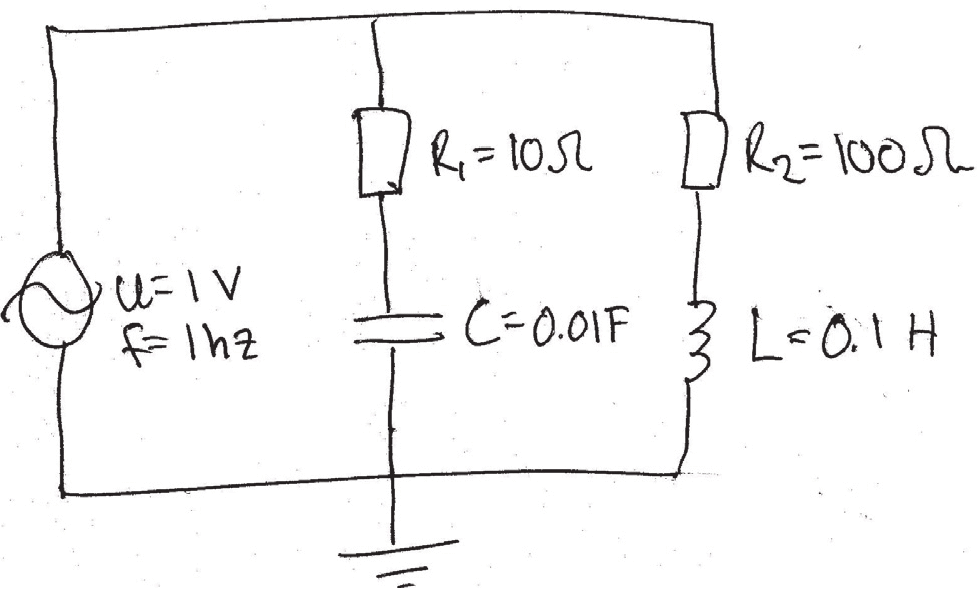
The draft schematics of an AC circuit model.
In this example, the circuit above will be used to illustrate the difference between a block-based approach and a component-based approach to modeling.
MODELS USED IN THIS TUTORIAL |
| ElectricCircuit BlockCircuit ElectricCircuit2 |
Block-Based Circuit
Begin by creating a block-based model. Before you actually start implementing the model, you have to:
In this example, you want to study the current through the sine voltage source in response to different frequencies of the driving voltage. To calculate this, you have three equations:
In these equations, i is the total current through the sine voltage source, and i1 and i2 are the currents running through resistor1 and resistor2, respectively. Rewrite the above equations to not contain derivatives:
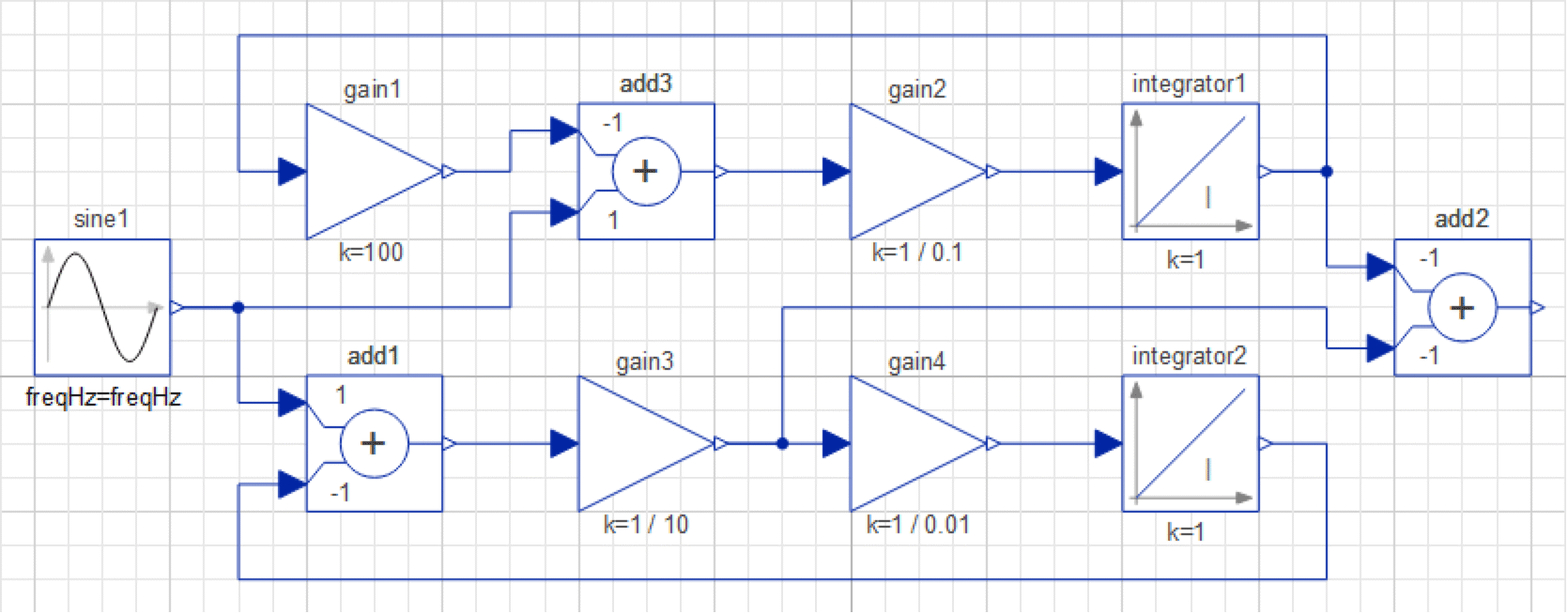
With these equations, you can now implement the block-based model, as shown below.
The Diagram View of the IntroductoryExamples.ComponentBased.BlockCircuit model.
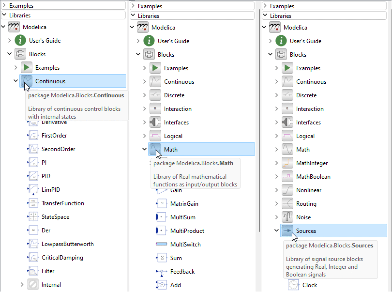
Create a new model and locate the components in the Class Browser. All components required to implement the system with a block-based approach can be found in the following packages:
To view the components in the Modelica.Blocks.Sources package in the Class Browser, expand the Modelica package, followed by Blocks and Sources, by clicking the symbol to the left of each package icon and name.
Expanding the Continuous, Math, and Sources packages within Modelica.Blocks.
Place the components in the Diagram View of your model by dragging them from the Class Browser and dropping them in the class window. Complete the model by connecting the components.
Switch to Simulation Center and simulate the model for 10 seconds. The output current is the result of add2. The signals i1 and i2 are from gain3 and integrator1, respectively. The picture below shows the resulting current.
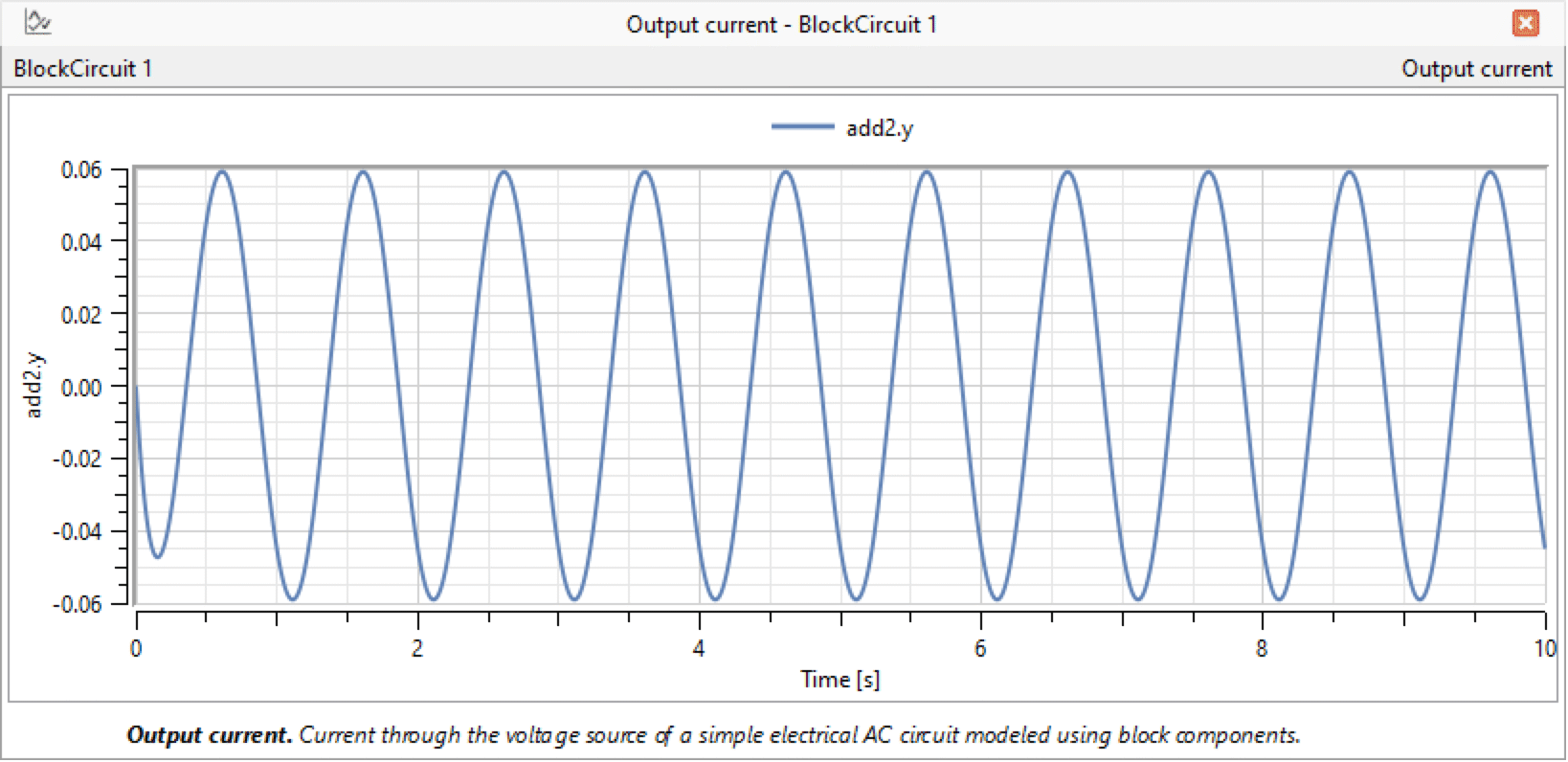
Plotting add2.y for the IntroductoryExamples.ComponentBased.BlockCircuit model with default parameter values.
Component-Based Circuit
Naturally, implementing a component-based model of the system shown in the original drawing requires only drag-and-drop, as well as connecting the components and setting parameters. This leaves us with a model that looks just like the drawing with which you started.
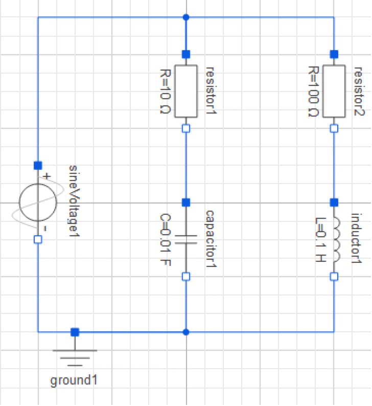
The Diagram View of the IntroductoryExamples.ComponentBased.ElectricCircuit model.
If you would like to build the model yourself, the sine voltage component is located in the Modelica.Electrical.Analog.Sources package, and the rest of the components in the Modelica.Electrical.Analog.Basic package. Note that some of the parameter values differ from the default, so in order to obtain the same simulation results you will have to change these as well.
Now you can simulate and plot the current sineVoltage1.i, and as expected it looks just like the result plotted from the block model.
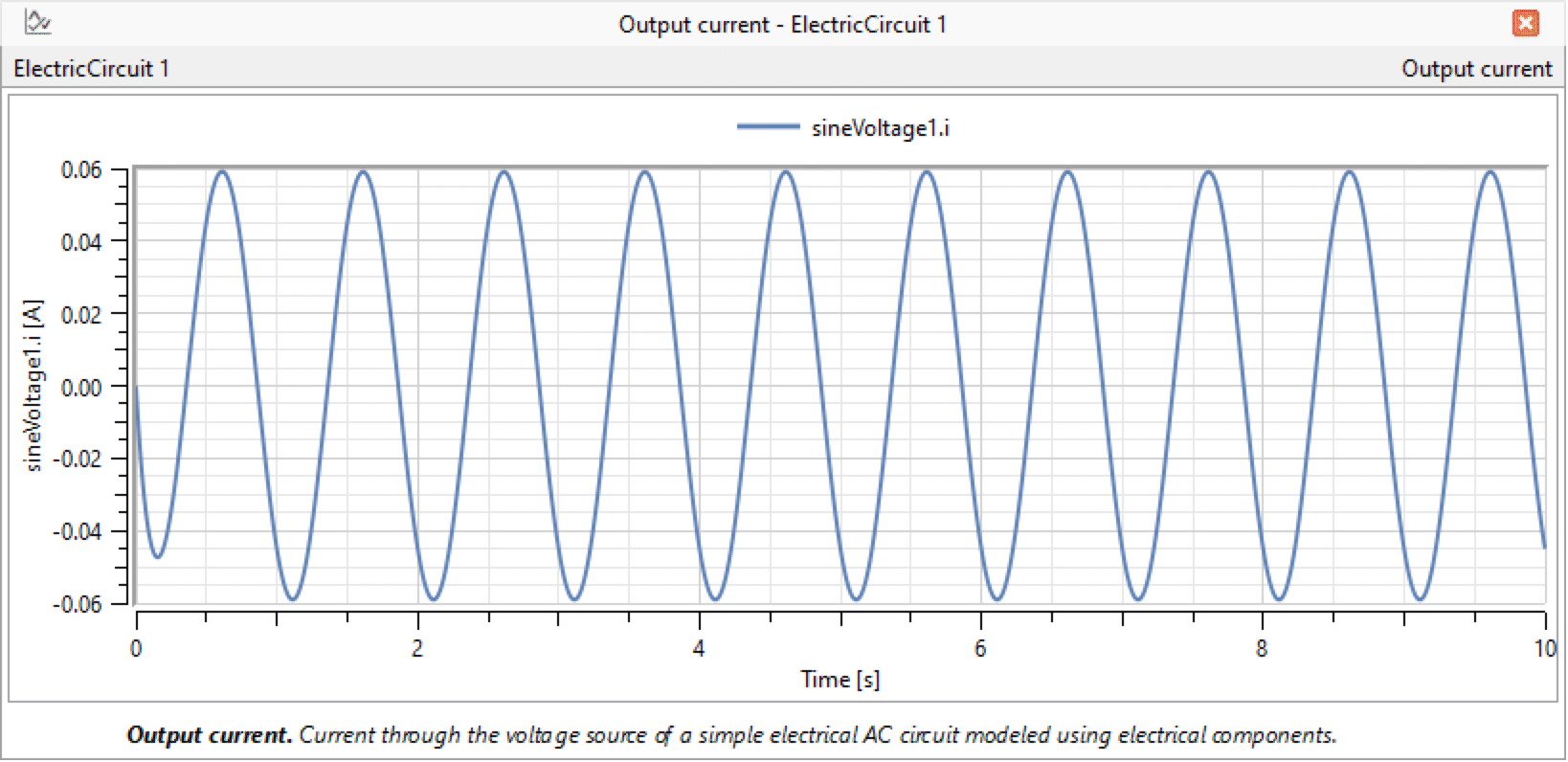
Plotting the current going through the sine voltage source for the IntroductoryExamples.ComponentBased.ElectricCircuit model with default parameter values.
You will end this section by adding a second capacitor to the model, as shown below. The capacitor component is located in the Modelica.Electrical.Analog.Basic package.
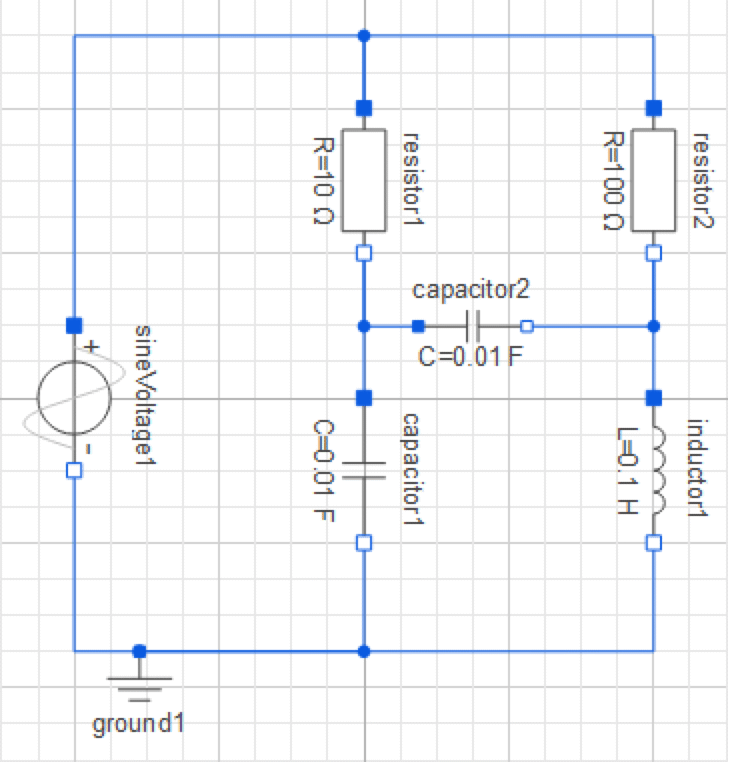
The Diagram View of the IntroductoryExamples.ComponentBased.ElectricCircuit2 model.
After simulation, you compare the resulting currents with one another.
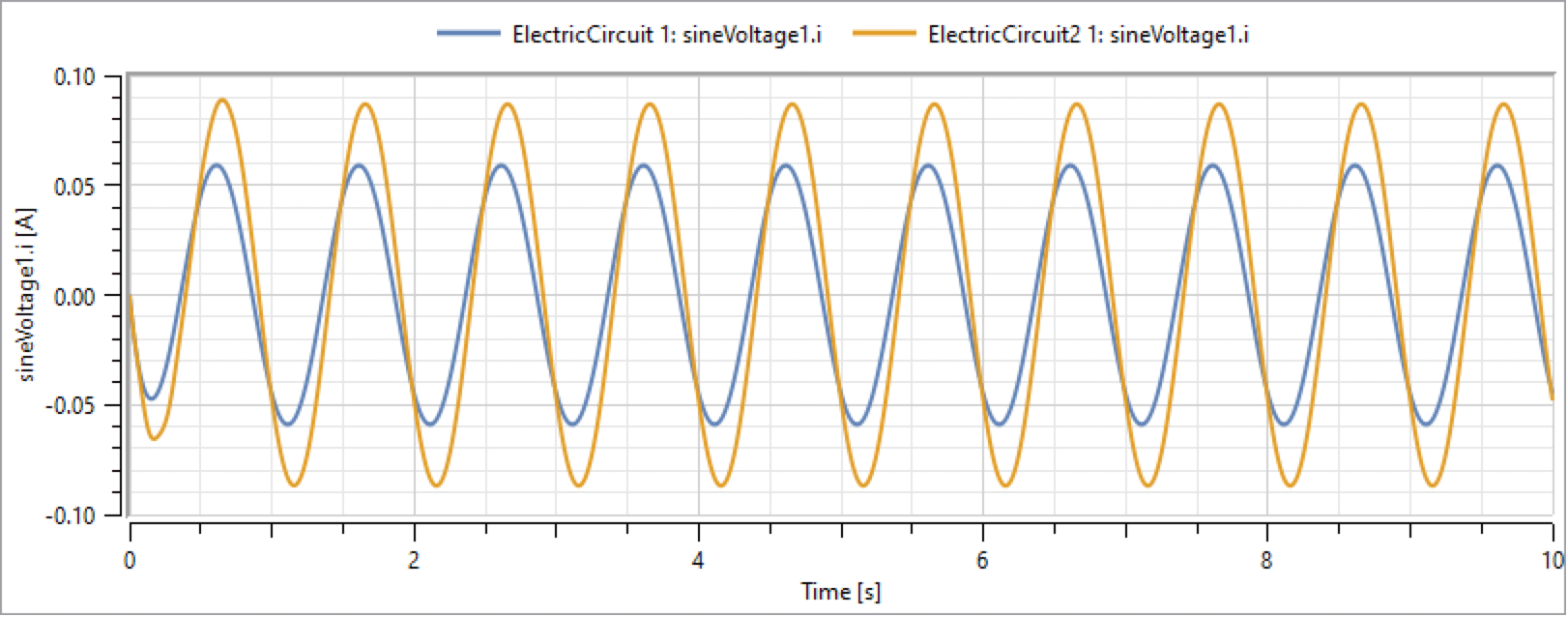
Comparison between the two currents going through the sine voltage source in the ElectricCircuit and ElectricCircuit2 models.
Exercise
Develop a block-based model for the second circuit.

