This information is part of the Modelica Standard Library maintained by the Modelica Association.

Calculation of pressure loss in curved bends at overall flow regime for incompressible and single-phase fluid flow through circular cross sectional area considering surface roughness.

Restriction

This function shall be used inside of the restricted limits according to the referenced literature.

• circular cross sectional area
• 0.5 ≤ curvature radius / diameter ≤ 3 [Idelchik 2006, p. 357, diag. 6-1]
• length of bend along curved axis / diameter ≥ 10 [Idelchik 2006, p. 357, diag. 6-1]
• angle of curvature smaller than 180° (delta ≤ 180) [Idelchik 2006, p. 357, diag. 6-1]

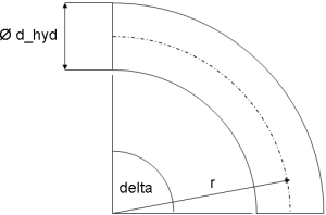
Geometry

Calculation

The pressure loss dp for curved bends is determined by:

dp = zeta_TOT * (rho/2) * velocity^2

with

rho	as density of fluid [kg/m3],
velocity	as mean velocity [m/s],
zeta_TOT	as pressure loss coefficient [-].

Curved bends with relative curvature radius R_0/d_hyd ≤ 3 according to [Idelchik 2006, p. 357, diag. 6-1]

The pressure loss of curved bends is similar to its calculation in straight pipes. There are three different flow regimes observed (laminar,transition,turbulent). The turbulent regime is further separated into sections with a dependence or independence of the local resistance coefficient (zeta_LOC) on Reynolds number. The local resistance coefficient (zeta_LOC) of a curved bend is calculated in dependence of the flow regime as follows:

• Laminar regime (Re ≤ Re_lam_leave):

  zeta_LOC = A2/Re + A1*B1*C1
  

• Transition regime (Re_lam_leave ≤ 4e4)

  This calculation is done using a smoothing function interpolating between the laminar and the first turbulent flow regime.

• Turbulent regime (4e4 ≤ 3e5) with dependence of local resistance coefficient on Reynolds number:

  zeta_LOC = k_Re * (A1*B1*C1)
  

  where k_Re depends on the relative curvature radius R_0/d_hyd

  k_Re = 1 + 4400/Re              for 0.50 < r/d_hyd < 0.55
  k_Re = 5.45/Re^(0.118)          for 0.55 ≤ r/d_hyd < 0.70
  k_Re = 11.5/Re^(0.19)           for 0.70 ≤ r/d_hyd < 3.00

• Turbulent regime (Re ≥ 3e5) with independence of local resistance coefficient on Reynolds number

  zeta_LOC = A1*B1*C1
  

with

A1	as coefficient considering effect of angle of turning (delta) [-],
A2	as coefficient considering effect for laminar regime [-],
B1	as coefficient considering effect of relative curvature radius (R_0/d_hyd) [-],
C1=1	as coefficient considering relative elongation of cross sectional area (here: circular cross sectional area) [-],
k_Re	as coefficient considering influence of laminar regime in transition regime [-],
Re	as Reynolds number [-].

The pressure loss coefficient zeta_TOT of a curved bend including pressure loss due to friction is determined by its local resistance coefficient zeta_LOC multiplied with a correction factor CF for surface roughness according to [Miller, p. 209, eq. 9.4]:

zeta_TOT = CF*zeta_LOC

where the correction factor CF is determined from the Darcy friction factor of a straight pipe having the bend flow path length

CF = 1 + (lambda_FRI_rough * pi * delta/d_hyd) / zeta_LOC

and the Darcy friction factors lambda_FRI_rough is calculated with an approximated Colebrook-White law according to [Miller, p. 191, eq. 8.4]:

lambda_FRI_rough = 0.25*(lg(K/(3.7*d_hyd) + 5.74/Re^0.9))^-2

with

delta	as curvature radiant [rad],
d_hyd	as hydraulic diameter [m],
K	as absolute roughness (average height of surface asperities) [m],
lambda_FRI_rough	as Darcy friction factor[-],
Re	as Reynolds number [m],
zeta_LOC	as local resistance coefficient [-],
zeta_TOT	as pressure loss coefficient [-].

The correction for surface roughness through CF is used only in the turbulent regime, where the fluid flow is influenced by surface asperities not covered by a laminar boundary layer. The turbulent regime starts at Re ≥ 4e4 according to [Idelchik 2006, p. 336, sec. 15]. There is no correction due to roughness in the laminar regime up to Re ≤ 6.5e3 according to [Idelchik 2006, p. 336, sec. 15].

Nevertheless the transition point from the laminar to the transition regime is shifted to smaller Reynolds numbers for an increasing absolute roughness. This effect is considered according to [Samoilenko in Idelchik 2006, p. 81, sec. 2-1-21] as:

Re_lam_leave = 754*exp(if k ≤ 0.007 then 0.0065/0.007 else 0.0065/k)

with

k = K /d_hyd	as relative roughness [-],
Re_lam_leave	as Reynolds number for leaving laminar regime [-].

Note that the beginning of the laminar regime cannot be beneath Re ≤ 1e2.

Verification

The pressure loss coefficient zeta_TOT of a curved bend in dependence of the Reynolds number Re for different relative curvature radii R_0/d_hyd and different angles of turning delta is shown in the figures below.

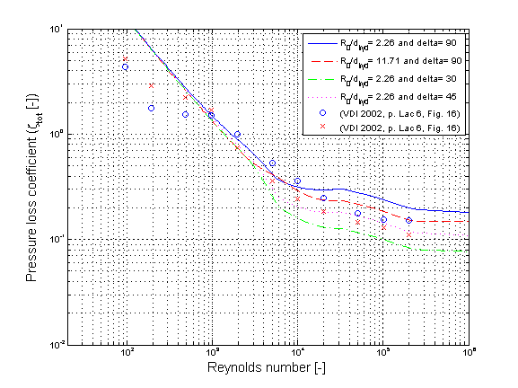
There are deviations of the pressure loss coefficient zeta_TOT comparing different references. Usually these deviations in the transition regime have to be accepted due to an uncertainty for the determination of comparable boundary conditions in the different references. Nevertheless these calculations cover the usual range of pressure loss coefficients for a curved bend. The pressure loss coefficient zeta_TOT for the same geometry can be adjusted via varying the average height of surface asperities K for calibration.

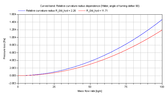
The pressure loss in dependence of the mass flow rate of water is shown for different relative curvature radii:

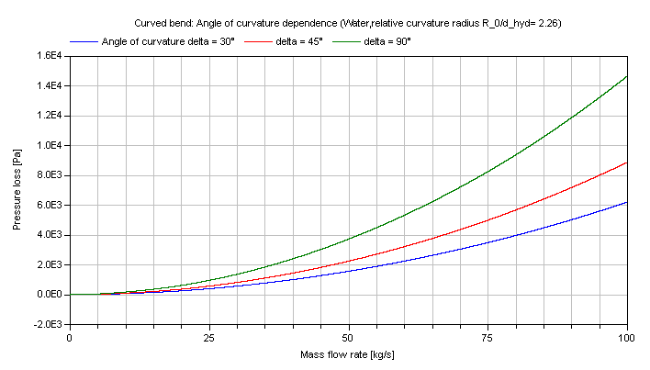
The pressure loss in dependence of the mass flow rate of water is shown for different angles of turning:

Note that there is a small deviation between the compressible and incompressible calculation due to the lack of a direct analytical invertibility.

References

Elmqvist,H., M.Otter and S.E. Cellier:

Inline integration: A new mixed symbolic / numeric approach for solving differential-algebraic equation systems.. In Proceedings of European Simulation MultiConference, Prague, 1995.

Idelchik,I.E.:

Handbook of hydraulic resistance. Jaico Publishing House, Mumbai, 3rd edition, 2006.

Miller,D.S.:

Internal flow systems. volume 5th of BHRA Fluid Engineering Series.BHRA Fluid Engineering, 1984.

Samoilenko,L.A.:

Investigation of the hydraulic resistance of pipelines in the zone of transition from laminar into turbulent motion. PhD thesis, Leningrad State University, 1968.

VDI:

VDI - Wärmeatlas: Berechnungsblätter für den Wärmeübergang. Springer Verlag, 9th edition, 2002.