WOLFRAM SYSTEM MODELER
dp_twoPhaseOverall |
|
Wolfram Language
In[1]:=

SystemModel["Modelica.Fluid.Dissipation.Utilities.SharedDocumentation.PressureLoss.StraightPipe.dp_twoPhaseOverall"]
Out[1]:=
Information
This information is part of the Modelica Standard Library maintained by the Modelica Association.
Calculation of pressure loss for two phase flow in a horizontal or vertical straight pipe for an overall flow regime considering frictional, momentum and geodetic pressure loss.
Restriction
This function shall be used within the restricted limits according to the referenced literature.
- circular cross sectional area
- neglecting of surface roughness
- horizontal flow or vertical upflow
- usage of mass flow rate quality (see Calculation)
- two phase pressure loss for mean constant mass flow rate quality (x_flow) over (increment) length
- usage of two phase pressure loss function for discretization at boiling or condensation considering variable mass flow rate quality
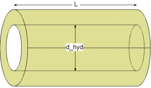
Geometry
Calculation
The two phase pressure loss dp_2ph of straight pipes is determined by:
dp_2ph = dp_fri + dp_mom + dp_geo
with
| dp_fri | as frictional pressure loss [Pa], |
| dp_mom | as momentum pressure loss [Pa], |
| dp_geo | as geodetic pressure loss [Pa]. |
Definition of quality for two phase flow:
Different definitions of the quality exist for two phase flow. Static quality, mass flow rate quality and thermodynamic quality can be used to describe the fraction of gas and liquid in two phase flow. Here the mass flow rate quality (x_flow) is used to describe two phase flow as follows:
x_flow = mdot_g/(mdot_g+mdot_l)
with
| x_flow | as mass flow rate quality [-], |
| mdot_g | as gaseous mass flow rate [kg/s], |
| mdot_l | as liquid mass flow rate [kg/s]. |
Note that mass flow rate quality (x_flow) is only equal to the static quality, if a difference between the velocity of gas and liquid phase is neglected (homogeneous approach). Additionally the thermodynamic quality is only equal to the mass flow rate quality (x_flow) in the two phase regime for thermodynamic equilibrium of the phases.
Frictional pressure loss:
The frictional pressure loss dp_fri of a straight pipe is calculated either by the correlation of Friedel (frictionalPressureLoss==Friedel) or by the correlation of Chisholm (frictionalPressureLoss==Chisholm). Both correlations can be used for the above named two phase flow regimes. The two phase frictional pressure loss results from a frictional pressure loss assuming one phase liquid fluid flow and a two phase multiplier taking into account the effects of two phase flow:
dp_fri = dp_1ph*phi_i
with
| dp_1ph | as frictional pressure loss assuming one phase liquid fluid flow [Pa], |
| phi_i | as two phase multiplier [-]. |
The liquid frictional pressure loss is calculated with the total mass flow rate assumed to flow as liquid.
The correlations of Friedel and Chisholm differ in their calculation of the two phase multiplier:
phi_friedel = (1 - x_flow)^2 + x_flow^2*(rho_l/rho_g)*(lambda_g/lambda_l)
            + 3.43*x_flow^0.685*(1 - x_flow)^0.24*(rho_l/rho_g)^0.8*(eta_g/eta_l)^0.22*(1 - eta_g/eta_l)^0.89*(1/Fr_l^(0.048))*(1/We_l^(0.0334))
phi_chisholm = 1 + (gamma^2 - 1)*(B*x_flow^((2 - n_exp)/2)*(1 - x_flow)^((2 -n_exp)/2) + x_flow^(2 - n_exp))
with
| B | as Lockhart-Martinelli coefficient [-], |
| eta_l | as dynamic viscosity of the liquid phase [Pas], |
| eta_g | as dynamic viscosity of the gaseous phase [Pas], |
| gamma | as physical property coefficient [-], |
| n_exp =0.2 | as exponent in Chisholm correlation [-], |
| phi_i | as two phase multiplier [-], |
| rho_l | as density of the liquid phase [kg/m3], |
| rho_g | as density of the gaseous phase [kg/m3], |
| Re_l | as Reynolds number of the liquid phase [-], |
| Re_g | as Reynolds number of the gaseous phase [-], |
| Fr_l | as Froude number of the liquid phase [-], |
| We_l | as Weber number of the liquid phase [-], |
| x_flow | as mass flow rate quality [-]. |
Note that the (mean constant) mass flow rate quality (x_flow) used for frictional pressure loss is calculated as arithmetic mean value out of the mass flow rate quality at the end and at the start of the straight pipe length.
Momentum pressure loss:
The momentum pressure loss dp_mom can be considered (momentumPressureLoss = true) for a homogeneous or heterogeneous two phase flow depending on the approach used for the void fraction (epsilon). At evaporation the liquid phase having a slow velocity has to be accelerated to the higher velocity of the gas. The difference in static pressure at the outlet and the inlet causes a positive momentum pressure loss at evaporation (assumed vice versa for condensation). The momentum pressure loss occurs for a changing mass flow rate quality due to condensation or evaporation according to [VDI 2006, p.Lba 4, eq. 22] :
dp_mom = mdot_A^2*[[((1-x_flow)^2/(rho_l*(1-epsilon)) + x_flow^2/(rho_g*epsilon))]_out - [((1-x_flow)^2/(rho_l*(1-epsilon)) + x_flow^2/(rho_g*epsilon))]_in]
with
| mdot_A | as total mass flow rate density [kg/(m2s)], |
| epsilon | as void fraction [-], |
| rho_l | as density of the liquid phase [kg/m3], |
| rho_g | as density of the gaseous phase [kg/m3], |
| x_flow | as mass flow rate quality [-]. |
Note that a momentum pressure loss is only considered for a variable mass flow rate quality (x_flow) during evaporation or condensation. Momentum pressure loss does not occur under adiabatic conditions for a corresponding constant mass flow rate quality (evaporation due to pressure loss is not considered).
Void fraction approach:
The void fraction is one of the most important parameter used to characterize two phase flow. There are several analytical and empirical approaches according to [Thome, J.R] :
- homogeneous approach
- momentum flux approach (heterogeneous model)
- Kinetic energy flow approach by Zivi (heterogeneous model)
- Empirical momentum flux approach by Chisholm (heterogeneous model)
These approaches for the void fraction epsilon imply a correlation for the slip ratio. The slip ratio is defined as ratio of the velocity from the gaseous phase to the liquid phase at two phase flow. The effects of different fluid flow velocities of the phases on two phase pressure loss can be considered with the slip ratio in the heterogeneous approaches. The slip ratio for the homogeneous approach is unity, so that there is no difference in the velocities of the two phases (e.g., usable for bubble flow).
Geodetic pressure loss:
The geodetic pressure loss dp_geo can be considered (geodeticPressureLoss=true) for two phase flow according to [VDI 2006, p.Lbb 1, eq. 4] :
dp_geo = (epsilon*rho_g +(1-epsilon)*rho_l)*g*L*sin(phi)
with
| epsilon | as void fraction [-], |
| rho_l | as density of the liquid phase [kg/m3], |
| rho_g | as density of the gaseous phase [kg/m3], |
| g | as acceleration of gravity [m/s2], |
| L | as length of straight pipe [m], |
| phi | as angle to horizontal [rad]. |
Verification
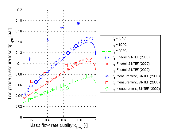
The two phase pressure loss for a horizontal pipe calculated by the correlation of Friedel neglecting momentum and geodetic pressure loss is shown in the figure below.
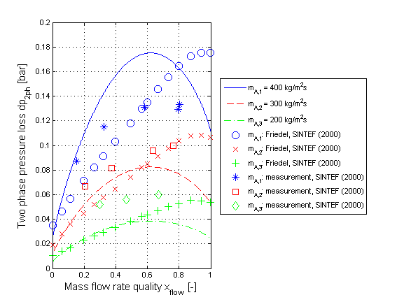
The two phase pressure loss for a horizontal pipe calculated by the correlation of Chisholm neglecting momentum and geodetic pressure loss is shown in the figure below.
References
- Chisholm,D.:
- Pressure gradients due to friction during the flow of evaporating two-phase mixtures in smooth tubes and channels. Volume 16th of International Journal of Heat and Mass Transfer, 1973.
- Friedel,L.:
- IMPROVED FRICTION PRESSURE DROP CORRELATIONS FOR HORIZONTAL AND VERTICAL TWO PHASE PIPE FLOW.3R International, Vol. 18, Issue 7, pp. 485-491, 1979.
- VDI:
- VDI - Wärmeatlas: Berechnungsblätter für den Wärmeübergang. Springer Verlag, 10th edition, 2006.
- J.M. Jensen and H. Tummescheit:
- Moving boundary models for dynamic simulations of two-phase flows. In Proceedings of the 2nd International Modelica Conference, pages 235-244, Oberpfaffenhofen, Germany, 2002. The Modelica Association.
- Thome, J.R.:
- Engineering Data Book 3.Swiss Federal Institute of Technology Lausanne (EPFL), 2009.