AsymptoticGreaterEqual[f,g,xx*]
gives conditions for ![]() or
or ![]() as xx*.
as xx*.
AsymptoticGreaterEqual[f,g,{x1,…,xn}{![]() ,…,
,…,![]() }]
}]
gives conditions for ![]() or
or ![]() as {x1,…,xn}{
as {x1,…,xn}{![]() ,…,
,…,![]() }.
}.


AsymptoticGreaterEqual
AsymptoticGreaterEqual[f,g,xx*]
gives conditions for ![]() or
or ![]() as xx*.
as xx*.
AsymptoticGreaterEqual[f,g,{x1,…,xn}{![]() ,…,
,…,![]() }]
}]
gives conditions for ![]() or
or ![]() as {x1,…,xn}{
as {x1,…,xn}{![]() ,…,
,…,![]() }.
}.
Details and Options
- Asymptotic greater or equal is also expressed as f is big-omega of g, f is lower bounded by g, f is of order at least g, and f grows at least as fast as g. The point x* is often assumed from context.
- Asymptotic greater or equal is an order relation and means
![TemplateBox[{{f, (, x, )}}, Abs]>=c TemplateBox[{{g, (, x, )}}, Abs]](Files/AsymptoticGreaterEqual.en/9.png "TemplateBox[{{f, (, x, )}}, Abs]>=c TemplateBox[{{g, (, x, )}}, Abs]") when x is near x* for some constant
when x is near x* for some constant  .
. - Typical uses include expressing simple lower bounds for functions and sequences near some point. It is frequently used for solutions to equations and to give simple lower bounds for computational complexity.
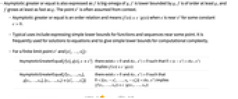
- For a finite limit point x* and {
 ,…,
,…, }:
}: -
AsymptoticGreaterEqual[f[x],g[x],xx*] there exist  and
and  such that
 ![0<TemplateBox[{{x, -, {x, ^, *}}}, Abs]<delta(c,x^*)](Files/AsymptoticGreaterEqual.en/15.png "0<TemplateBox[{{x, -, {x, ^, *}}}, Abs]<delta(c,x^*)") implies
implies ![TemplateBox[{{f, (, x, )}}, Abs]>=c TemplateBox[{{g, (, x, )}}, Abs]](Files/AsymptoticGreaterEqual.en/16.png "TemplateBox[{{f, (, x, )}}, Abs]>=c TemplateBox[{{g, (, x, )}}, Abs]")
AsymptoticGreaterEqual[f[x1,…,xn],g[x1,…,xn],{x1,…,xn}{  ,…,
,…, }]
}]there exist  and
and  such that
 ![0<TemplateBox[{{{, {{{x, _, 1}, -, {x, _, 1, ^, *}}, ,, ..., ,, {{x, _, n}, -, {x, _, n, ^, *}}}, }}}, Norm]<delta(epsilon,x^*)](Files/AsymptoticGreaterEqual.en/21.png "0<TemplateBox[{{{, {{{x, _, 1}, -, {x, _, 1, ^, *}}, ,, ..., ,, {{x, _, n}, -, {x, _, n, ^, *}}}, }}}, Norm]<delta(epsilon,x^*)") implies
implies ![TemplateBox[{{f, (, {{x, _, 1}, ,, ..., ,, {x, _, n}}, )}}, Abs]>=c TemplateBox[{{g, (, {{x, _, 1}, ,, ..., ,, {x, _, n}}, )}}, Abs]](Files/AsymptoticGreaterEqual.en/22.png "TemplateBox[{{f, (, {{x, _, 1}, ,, ..., ,, {x, _, n}}, )}}, Abs]>=c TemplateBox[{{g, (, {{x, _, 1}, ,, ..., ,, {x, _, n}}, )}}, Abs]")
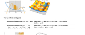
- For an infinite limit point:
-
AsymptoticGreaterEqual[f[x],g[x],x∞] there exist  and
and  such that
  implies
 ![TemplateBox[{{f, (, x, )}}, Abs]>=c TemplateBox[{{g, (, x, )}}, Abs]](Files/AsymptoticGreaterEqual.en/27.png "TemplateBox[{{f, (, x, )}}, Abs]>=c TemplateBox[{{g, (, x, )}}, Abs]")
AsymptoticGreaterEqual[f[x1,…,xn],g[x1,…,xn],{x1,…,xn}{∞,…,∞}] there exist  and
and  such that
  implies
 ![TemplateBox[{{f, (, {{x, _, 1}, ,, ..., ,, {x, _, n}}, )}}, Abs]>=c TemplateBox[{{g, (, {{x, _, 1}, ,, ..., ,, {x, _, n}}, )}}, Abs]](Files/AsymptoticGreaterEqual.en/31.png "TemplateBox[{{f, (, {{x, _, 1}, ,, ..., ,, {x, _, n}}, )}}, Abs]>=c TemplateBox[{{g, (, {{x, _, 1}, ,, ..., ,, {x, _, n}}, )}}, Abs]")
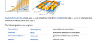
- AsymptoticGreaterEqual[f[x],g[x],xx*] exists if and only if MinLimit[Abs[f[x]/g[x]],xx*]>0 when g[x] does not have an infinite set of zeros near x*.
- The following options can be given:
-
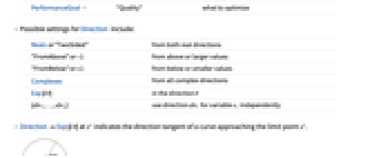
Assumptions $Assumptions assumptions on parameters Direction Reals direction to approach the limit point GenerateConditions Automatic generate conditions for parameters Method Automatic method to use PerformanceGoal "Quality" what to optimize - Possible settings for Direction include:
-
Reals or "TwoSided" from both real directions "FromAbove" or -1 from above or larger values "FromBelow" or +1 from below or smaller values Complexes from all complex directions Exp[ θ] in the direction 
{dir1,…,dirn} use direction diri for variable xi independently - DirectionExp[ θ] at x* indicates the direction tangent of a curve approaching the limit point x*.
- Possible settings for GenerateConditions include:
-
Automatic non-generic conditions only True all conditions False no conditions None return unevaluated if conditions are needed - Possible settings for PerformanceGoal include $PerformanceGoal, "Quality" and "Speed". With the "Quality" setting, Limit typically solves more problems or produces simpler results, but it potentially uses more time and memory.
Examples
open all close allBasic Examples (2)
Scope (9)
Compare functions that are not strictly positive:
Show that ![]() diverges at least as fast as
diverges at least as fast as ![]() at the origin:
at the origin:
Answers may be Boolean expressions rather than explicit True or False:
When comparing functions with parameters, conditions for the result may be generated:
By default, a two-sided comparison of the functions is made:
When comparing larger values of ![]() ,
, ![]() is indeed no smaller than
is indeed no smaller than ![]() :
:
The relationship fails for smaller values of ![]() :
:
Functions like Sqrt may have the same relationship in both real directions along the negative reals:
If approached from above in the complex plane, the same relationship is observed:
However, approaching from below in the complex plane produces a different result:
This is due to a branch cut where the imaginary part of Sqrt reverses sign as the axis is crossed:
Hence, the relationship does not hold in the complex plane in general:
Visualize the relative sizes of the functions when approached from the four real and imaginary directions:
Compare multivariate functions:
Visualize the norms of the two functions:
Options (10)
Assumptions (1)
Specify conditions on parameters using Assumptions:
Direction (5)
Test the relation at piecewise discontinuities:
Since it fails in one direction, the two-sided result is false as well:
Visualize the two functions and their ratio:
The relationship at a simple pole is independent of the direction of approach:
Test the relation at a branch cut:
Compute the relation, approaching from different quadrants:
Approaching the origin from the first quadrant:
Approaching the origin from the fourth quadrant:
Approach the origin from the right half-plane:
Approaching the origin from the bottom half-plane:
Visualize the ratio of the functions, which becomes large near the origin except along ![]() :
:
GenerateConditions (3)
Return a result without stating conditions:
This result is only valid if n>0:
Return unevaluated if the results depend on the value of parameters:
By default, conditions are generated that guarantee a result:
By default, conditions are not generated if only special values invalidate the result:
With GenerateConditions->True, even these non-generic conditions are reported:
PerformanceGoal (1)
Use PerformanceGoal to avoid potentially expensive computations:
The default setting uses all available techniques to try to produce a result:
Applications (10)
Basic Applications (4)
Computational Complexity (4)
Simple sorting algorithms (bubble sort, insertion sort) take approximately a n2 steps to sort n objects, while optimal general algorithms (heap sort, merge sort) take approximately b n Log[n] steps to do the sort. Show that ![]() , so that optimal algorithms are never slower for large enough collections of objects:
, so that optimal algorithms are never slower for large enough collections of objects:
Certain special algorithms (counting sort, radix sort), where there is information ahead of time about the possible inputs, can run in c n time. Show that ![]() :
:
Visualize the growth of the three time scales:
In a bubble sort, adjoining neighbors are compared and swapped if they are out of order. After one pass of n-1 comparisons, the largest element is at the end. The process is then repeated on remaining n-1 elements, and so forth, until only two elements at the very beginning remain. If comparison and swap takes c steps, the total number of steps for the sort is as follows:
Thus ![]() , and the algorithm is said to have quadratic run time:
, and the algorithm is said to have quadratic run time:
In a merge sort, the list of elements is split in two, each half is sorted, and then the two halves are combined. Thus, the time T[n] to do the sort will be the sum of some constant time b to compute the middle, 2T[n/2] to sort each half, and some multiple a n of the number of elements to combine the two halves:
Solve the recurrence equation to find the time t to sort n elements:
Hence ![]() , and the algorithm is said to have
, and the algorithm is said to have ![]() run time:
run time:
The traveling salesperson problem (TSP) consists of finding the shortest route connecting ![]() cities. A naive algorithm is to try all
cities. A naive algorithm is to try all ![]() routes. The Held–Karp algorithm improves that to roughly
routes. The Held–Karp algorithm improves that to roughly ![]() steps. Show that
steps. Show that ![]() :
:
Both algorithms show that the complexity class of TSP is no worse than EXPTIME, which are problems that can be solved in time ![]() . For Held–Karp, using
. For Held–Karp, using ![]() for some
for some ![]() suffices:
suffices:
For the factorial, it is necessary to use a higher-degree polynomial, for example ![]() :
:
Approximate solutions can be found in ![]() time, so the approximate TSP is in the complexity class P of problems solvable in polynomial time. Any polynomial algorithm is faster than an exponential one, or
time, so the approximate TSP is in the complexity class P of problems solvable in polynomial time. Any polynomial algorithm is faster than an exponential one, or ![]() :
:
Convergence Testing (2)
A sequence ![]() is said to be absolutely summable if
is said to be absolutely summable if ![]() . If a second sequence
. If a second sequence ![]() and
and ![]() is not absolutely summable, the comparison test states that
is not absolutely summable, the comparison test states that ![]() is not absolutely summable either. Use the test to show that
is not absolutely summable either. Use the test to show that ![]() diverges by comparing with the sum of
diverges by comparing with the sum of ![]() :
:
Since the harmonic series diverges, so does ![]() :
:
Compare with the answer given by SumConvergence:
Another sequence comparable to ![]() is
is ![]() , and thus it is not absolutely summable either:
, and thus it is not absolutely summable either:
Show that the sequence ![]() , and thus cannot be absolutely summable:
, and thus cannot be absolutely summable:
Compare with the answer given by SumConvergence:
A function ![]() is said to be absolutely integrable on
is said to be absolutely integrable on ![]() if
if ![]() . If
. If ![]() and
and ![]() are continuous on the open interval
are continuous on the open interval ![]() and
and ![]() at both
at both ![]() and
and ![]() , the comparison test states that if
, the comparison test states that if ![]() is not absolutely integrable, then
is not absolutely integrable, then ![]() is not as well. Use the test to show that
is not as well. Use the test to show that ![]() is not absolutely integrable on
is not absolutely integrable on ![]() :
:
Since ![]() and
and ![]() is not integrable on
is not integrable on ![]() , neither is
, neither is ![]() :
:
The function ![]() is not absolutely integrable on
is not absolutely integrable on ![]() :
:
At both ![]() and
and ![]() ,
, ![]() , and hence the nonintegrability of
, and hence the nonintegrability of ![]() follows:
follows:
Show that these functions are not absolutely integrable over ![]() because
because ![]() is not:
is not:
For ![]() ,
, ![]() , so the comparison test gives no information about convergence:
, so the comparison test gives no information about convergence:
Properties & Relations (8)
AsymptoticGreaterEqual is a reflexive relation, i.e. ![]() :
:
And it is a transitive relation, i.e. ![]() and
and ![]() implies
implies ![]() :
:
However, it is not symmetric, i.e. ![]() does not imply
does not imply ![]() :
:
AsymptoticGreaterEqual[f[x],g[x],xx0] iff MinLimit[Abs[f[x]/g[x]],xx0]>0:
AsymptoticGreaterEqual[f[x],g[x],xx0] if Limit[Abs[f[x]/g[x]],xx0]>0:
However, when the limit is Indeterminate, it is inconclusive:
Text
Wolfram Research (2018), AsymptoticGreaterEqual, Wolfram Language function, https://reference.wolfram.com/language/ref/AsymptoticGreaterEqual.html.
CMS
Wolfram Language. 2018. "AsymptoticGreaterEqual." Wolfram Language & System Documentation Center. Wolfram Research. https://reference.wolfram.com/language/ref/AsymptoticGreaterEqual.html.
APA
Wolfram Language. (2018). AsymptoticGreaterEqual. Wolfram Language & System Documentation Center. Retrieved from https://reference.wolfram.com/language/ref/AsymptoticGreaterEqual.html