


Limit
Details and Options

- Limit is also known as function limit, directed limit, iterated limit, nested limit and multivariate limit.
- Limit computes the limiting value f* of a function f as its variables x or xi get arbitrarily close to their limiting point x* or
 .
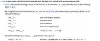
. - By using the character , entered as
 lim
lim or \[Limit], with underscripts or subscripts, limits can be entered as follows:
 -
 f
flimit in the default direction  f
flimit from above  f
flimit from below  f
flimit in the complex plane  …
… f
fLimit[f,{x1  ,…,xn
,…,xn }]
}] - For a finite limit point x* and {
 ,…,
,…, } and finite limit value f*:
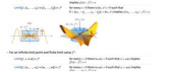
 -
Limit[f,xx*]f* for every  there is
  such that
 ![0<TemplateBox[{{x, -, {x, ^, *}}}, Abs]<delta(epsilon,x^*)](Files/Limit.en/27.png "0<TemplateBox[{{x, -, {x, ^, *}}}, Abs]<delta(epsilon,x^*)") implies
implies ![TemplateBox[{{{f, (, x, )}, -, {f, ^, *}}}, Abs]<epsilon](Files/Limit.en/28.png "TemplateBox[{{{f, (, x, )}, -, {f, ^, *}}}, Abs]<epsilon")
Limit[f,{x1,…,xn}{  ,…,
,…, }]f*
}]f*for every  there is
  such that
 ![0<TemplateBox[{{{, {{{x, _, 1}, -, {x, _, {(, 1, )}, ^, *}}, ,, ..., ,, {{x, _, n}, -, {x, _, {(, n, )}, ^, *}}}, }}}, Norm]<delta(epsilon,x^*)](Files/Limit.en/33.png "0<TemplateBox[{{{, {{{x, _, 1}, -, {x, _, {(, 1, )}, ^, *}}, ,, ..., ,, {{x, _, n}, -, {x, _, {(, n, )}, ^, *}}}, }}}, Norm]<delta(epsilon,x^*)") implies
implies ![TemplateBox[{{{f, (, {{x, _, 1}, ,, ..., ,, {x, _, n}}, )}, -, {f, ^, *}}}, Abs]<epsilon](Files/Limit.en/34.png "TemplateBox[{{{f, (, {{x, _, 1}, ,, ..., ,, {x, _, n}}, )}, -, {f, ^, *}}}, Abs]<epsilon")
- For an infinite limit point and finite limit value f*:
-
Limit[f,x∞]f* for every  there is
  such that
  implies
 ![TemplateBox[{{{f, (, x, )}, -, {f, ^, *}}}, Abs]<epsilon](Files/Limit.en/39.png "TemplateBox[{{{f, (, x, )}, -, {f, ^, *}}}, Abs]<epsilon")
Limit[f,{x1,…,xn}{∞,…,∞}]f* for every  there is
  such that
  implies
 ![TemplateBox[{{{f, (, {{x, _, 1}, ,, ..., ,, {x, _, n}}, )}, -, {f, ^, *}}}, Abs]<epsilon](Files/Limit.en/43.png "TemplateBox[{{{f, (, {{x, _, 1}, ,, ..., ,, {x, _, n}}, )}, -, {f, ^, *}}}, Abs]<epsilon")
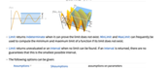
- Limit returns Indeterminate when it can prove the limit does not exist. MinLimit and MaxLimit can frequently be used to compute the minimum and maximum limit of a function if its limit does not exist.
- Limit returns unevaluated or an Interval when no limit can be found. If an Interval is returned, there are no guarantees that this is the smallest possible interval.
- The following options can be given:
-
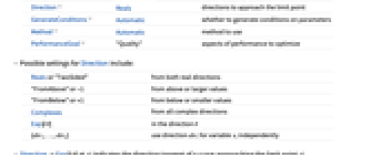
Assumptions $Assumptions assumptions on parameters Direction Reals directions to approach the limit point GenerateConditions Automatic whether to generate conditions on parameters Method Automatic method to use PerformanceGoal "Quality" aspects of performance to optimize - Possible settings for Direction include:
-
Reals or "TwoSided" from both real directions "FromAbove" or -1 from above or larger values "FromBelow" or +1 from below or smaller values Complexes from all complex directions Exp[ θ] in the direction 
{dir1,…,dirn} use direction diri for variable xi independently - DirectionExp[ θ] at x* indicates the direction tangent of a curve approaching the limit point x*.
- Possible settings for GenerateConditions include:
-
Automatic non-generic conditions only True all conditions False no conditions None return unevaluated if conditions are needed - Possible settings for PerformanceGoal include $PerformanceGoal, "Quality" and "Speed". With the "Quality" setting, Limit typically solves more problems or produces simpler results, but it potentially uses more time and memory.
Examples
open all close allBasic Examples (3)
Scope (35)
Basic Uses (5)
Find the limit at a symbolic point:
Find the limit at -Infinity:
The nested limit as ![]() first and then
first and then ![]() :
:
Typeset Limits (4)
Use ![]() lim
lim![]() to enter the character, and
to enter the character, and ![]() to create an underscript:
to create an underscript:
Take a limit from above or below by using a superscript ![]() or
or ![]() on the limit point:
on the limit point:
After typing zero, use ![]() to create a superscript:
to create a superscript:
To specify a direction of Reals or Complexes, enter the domain as an underscript on the character:
Enter the rule as ![]() ->
->![]() , use
, use ![]() to create an underscript, and type
to create an underscript, and type ![]() reals
reals![]() to enter
to enter ![]() :
:
TraditionalForm formatting:
Elementary Functions (6)
Polynomial and rational functions:
The function ![]() approaches positive infinity from both sides of
approaches positive infinity from both sides of ![]() :
:
The limit does not exist as the function approaches a different infinity on each side of ![]() :
:
A trigonometric function with a vertical asymptote:
A wildly oscillatory function with no limit at the origin:
Functions like Sqrt and Log have a two-sided limit along the negative reals:
If approached from above in the complex plane, the same limit value is reached:
However, approaching from below in the complex plane produces a different limit value:
This is due to branch cut where the imaginary part reverses sign as the axis is crossed:
Elementary Functions at Infinity (4)
Piecewise Functions (5)
A discontinuous piecewise function:
The value of the function at ![]() lies away from the nearby values of the function as
lies away from the nearby values of the function as ![]() :
:
A left-continuous piecewise function:
The function is left continuous because ![]() agrees with the limit as
agrees with the limit as ![]() from the left:
from the left:
UnitStep is effectively a right-continuous piecewise function:
It is right continuous because ![]() agrees with the limit as
agrees with the limit as ![]() from the right:
from the right:
RealSign is effectively a discontinuous piecewise function:
The value of ![]() disagrees with the limit as
disagrees with the limit as ![]() from both the left and right:
from both the left and right:
Find the limit of Floor as x approaches from larger numbers:
Find the limit of Floor as x approaches from smaller numbers:
Special Functions (4)
Nested Limits (3)
Compute the nested limit as first ![]() and then
and then ![]() :
:
The same result is obtained by computing two Limit expressions:
Computing the limit as first ![]() and then
and then ![]() yields a different answer:
yields a different answer:
This is again equivalent to two nested limits:
The nested limit as first ![]() and then
and then ![]() is
is ![]() :
:
The nested limit as first ![]() and then
and then ![]() is
is ![]() :
:
Consider the function for two variables at the origin:
The iterated limit as ![]() and then
and then ![]() is
is ![]() :
:
The iterated limit as ![]() and then
and then ![]() is
is ![]() :
:
Since the value of the limit depends on the order, the bivariate limit does not exist:
Visualize the function and the values along the two axes computed previously:
Multivariate Limits (4)
Compute the bivariate limit of a function as ![]() :
:
The limit value is ![]() if for all
if for all ![]() , there is a
, there is a ![]() where
where ![]() implies
implies ![]() :
:
For this function, the value ![]() will suffice:
will suffice:
The function lies in between the two cones with slope ![]() :
:
Find the limit of a multivariate function:
Various iterated limits exist:
Approaching the origin along the curve ![]() yields a third result:
yields a third result:
The true two-dimensional limit of the function does not exist:
Visualize the limit near the origin:
Find the limit of a bivariate function at the origin:
The true two-dimensional limit at the origin is zero:
Re-express the function in terms of polar coordinates:
The polar expression is bounded, and the limit as ![]() is:
is:
Compute the limit of a trivariate function:
The limit at the origin does not exist:
Limits in the ![]() and
and ![]() planes do exist:
planes do exist:
Options (13)
Assumptions (2)
Specify conditions on parameters using Assumptions:
Direction (5)
GenerateConditions (3)
Return a result without stating conditions:
This result is only valid if n>0:
Return unevaluated if the results depend on the value of parameters:
By default, conditions are generated that return a unique result:
By default, conditions are not generated if only special values invalidate the result:
With GenerateConditions->True, even these non-generic conditions are reported:
Method (2)
PerformanceGoal (1)
Use PerformanceGoal to avoid potentially expensive computations:
The default setting uses all available techniques to try to produce a result:
Applications (23)
Geometry of Limits (5)
The limit of the function ![]() as
as ![]() is
is ![]() :
:
This means that for values of ![]() close to
close to ![]() ,
, ![]() has a value close to
has a value close to ![]() :
:
The limit makes no statement about the value of ![]() at
at ![]() , which in this case is indeterminate:
, which in this case is indeterminate:
The function ![]() does not have a limit as
does not have a limit as ![]() approaches
approaches ![]() :
:
The function ![]() has the limit zero:
has the limit zero:
In increasingly small regions around ![]() ,
, ![]() continually bounces between
continually bounces between ![]() , but
, but ![]() gets increasingly flat:
gets increasingly flat:
The following rational function has a finite limit as ![]() :
:
Compute the ![]() that ensures that
that ensures that ![]() whenever
whenever ![]() :
:
The complicated result can be simplified by focusing on ![]() in the range between 0 and 2:
in the range between 0 and 2:
The plot of ![]() always "leaves" the rectangle of height
always "leaves" the rectangle of height ![]() and width
and width ![]() centered
centered ![]() through the sides, not the top or bottom:
through the sides, not the top or bottom:
Find vertical and horizontal asymptotes of a rational function:
Compute where the denominator is zero:
Verify that the function approaches ![]() at the computed values:
at the computed values:
Visualize the function and its asymptotes:
Find the non-vertical, linear asymptote of a function:
Discontinuities (5)
Classify the continuity or discontinuity of f at the origin:
It is not defined at 0, so it cannot be continuous:
Moreover, the limit as x0 does not exist:
However, the limit from below exists:
The limit from above also exists, but has a different value:
Therefore, f has a jump discontinuity at 0:
Classify the continuity or discontinuity of f at the origin:
The two-sided limit exists but does not equal the function value, so this is a removable discontinuity:
Find and classify the discontinuities of a piecewise function:
The function is not defined at zero so it cannot be continuous there:
The function tends to Infinity (on both sides), so this is an infinite discontinuity:
Next find where the limit does not equal the function:
The limit does exist at x==3, so this is a removable discontinuity:
The function ![]() is discontinuous at every multiple of
is discontinuous at every multiple of ![]() :
:
For example, at the origin it gives rise to the indeterminate form ![]() :
:
At every even multiple of ![]() , the two-sided limit of
, the two-sided limit of ![]() exists:
exists:
This is also true at the odd multiples of ![]() , with a different limit:
, with a different limit:
However, at the half-integer multiples of ![]() , the two sided limit does not exist:
, the two sided limit does not exist:
The function ![]() agrees with
agrees with ![]() where both are defined, but it is also continuous at multiples of
where both are defined, but it is also continuous at multiples of ![]() :
:
Show that ![]() is continuous at the origin:
is continuous at the origin:
Determine whether the following function is continuous at the origin, and whether limits along rays exist:
The bivariate limit does not exist, so the function is not continuous:
The limit in the left half-plane exists and is zero, so any ray approaching from there has the same limit:
Approaching along the line ![]() with
with ![]() gives a result in terms of the slope:
gives a result in terms of the slope:
Derivatives (5)
Compute the derivative of ![]() using the definition of derivative:
using the definition of derivative:
First compute the difference quotient:
The derivative is the limit as ![]() of the difference quotient:
of the difference quotient:
Compute the derivative of ![]() at
at ![]() :
:
The limit of the difference quotient does not exist, so ![]() is not differentiable at the origin:
is not differentiable at the origin:
Note that the left and right limits of the difference quotient exist but are unequal:
In this case, the left and right derivatives equal the limits of ![]() from the left and right:
from the left and right:
Visualize ![]() and its derivative; the former has a "kink" at zero, the latter a jump discontinuity:
and its derivative; the former has a "kink" at zero, the latter a jump discontinuity:
Determine the differentiability of ![]() at
at ![]() :
:
The limit of the difference quotient exists, so ![]() is differentiable and
is differentiable and ![]() :
:
Note that the limit as ![]() of
of ![]() does not exist, so
does not exist, so ![]() is discontinuous:
is discontinuous:
Determine the differentiability of ![]() at the point
at the point ![]() :
:
The partial derivative with respect to x exists:
As does the one with respect to y:
However, the linearization condition ![]() fails, so
fails, so ![]() is not differentiable:
is not differentiable:
Note that the partial derivatives of ![]() exist everywhere:
exist everywhere:
But they are discontinuous at the point ![]() :
:
The derivative is defined as the limit of the difference quotient:
The second derivative can be computed by taking the limit of the second-order difference quotient:
Directly compute the mixed partial derivative ![]() by taking a limit:
by taking a limit:
Mathematical Constants and Expressions (4)
Compute ![]() as a limit at Infinity:
as a limit at Infinity:
The complementary limit at the origin:
Compute ![]() as a limit of Gamma functions:
as a limit of Gamma functions:
Compute EulerGamma as a limit involving the Zeta function:
Compute EulerGamma as a limit of exponential integrals:
Other Applications (4)
A function ![]() is said to be "little-o of
is said to be "little-o of ![]() " at
" at ![]() , written
, written ![]() , if
, if ![]() :
:
Similarly, ![]() is said to be "little-omega of
is said to be "little-omega of ![]() ", written
", written ![]() , if
, if ![]() :
:
It is possible for two functions to share neither relationship:
Moreover, neither relationship even holds between a function and itself:
Hence, ![]() and
and ![]() define partial orders on the functions:
define partial orders on the functions:
![]() denotes the opposite relationship:
denotes the opposite relationship:
Note that the two lists are not exactly reversed, because ![]() and
and ![]() are incomparable:
are incomparable:
From Taylor's theorem, if ![]() has
has ![]() continuous derivatives around
continuous derivatives around ![]() , then
, then ![]() :
:
This is the fifth-order Taylor polynomial at ![]() :
:
In special relativity, the kinetic energy of a particle of mass ![]() and speed
and speed ![]() is given by:
is given by:
The classical formula for kinetic energy is:
In the limit that the speed approaches zero, these two formulas agree:
Properties & Relations (14)
Multiplicative constants can be moved outside a limit:
If f and g have finite limits, Limit is distributive over their sum:
If f and g have finite limits, Limit is distributive over their product:
Powers can be moved outside a limit:
Function composition and sequence limit operations can be interchanged for continuous functions:
This need not hold for discontinuous functions:
The "squeezing" or "sandwich" theorem:
The limit of the bounding functions is zero, which proves the original limit was zero:
The squeezing theorem for limits at infinity:
This function is bounded by ![]() on the positive real axis:
on the positive real axis:
The limit of the bounding functions is zero, which proves the original limit was zero:
Assumptions applies to parameters in the limit expression:
Direction places conditions on the limit variable:
Derivatives are defined in terms of limits:
The limit of a ratio can often be computed using L'Hôpital's rule:
Computing the ratio directly gives an indeterminate form 0/0:
The limit of the ratio equals the limit of the ratio of the derivatives:
In this case, f' and g' are continuous and can be computed via evaluation:
If Limit exists, then so does DiscreteLimit, and they have the same value:
If Limit exists, then so does MaxLimit, and it has the same value:
If Limit exists, then so does MinLimit, and it has the same value:
At each point of the domain, the limit of a continuous function is equal to its value:
Use FunctionContinuous to test whether a function is continuous:
Possible Issues (1)
Limit may return an incorrect answer for an inexact input:
Interactive Examples (1)
Text
Wolfram Research (1988), Limit, Wolfram Language function, https://reference.wolfram.com/language/ref/Limit.html (updated 2017).
CMS
Wolfram Language. 1988. "Limit." Wolfram Language & System Documentation Center. Wolfram Research. Last Modified 2017. https://reference.wolfram.com/language/ref/Limit.html.
APA
Wolfram Language. (1988). Limit. Wolfram Language & System Documentation Center. Retrieved from https://reference.wolfram.com/language/ref/Limit.html