DiffusionPDETerm
DiffusionPDETerm[vars]
represents a diffusion term ![]() with model variables vars.
with model variables vars.
DiffusionPDETerm[vars,c]
represents a diffusion term ![]() with diffusion coefficient
with diffusion coefficient ![]() .
.
DiffusionPDETerm[vars,c,pars]
uses model parameters pars.
Details


- Diffusion is a central concept of physics that is used in a number of domains, such as thermodynamics, acoustics, structural mechanics and fluid dynamics.
- Diffusion is also known as conduction.
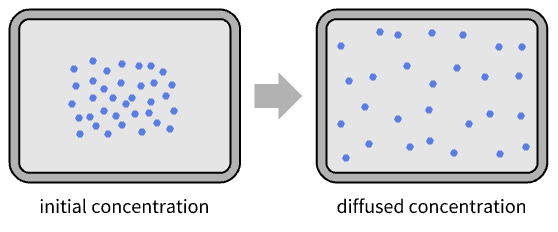
- Diffusion with a diffusion coefficient
 is the process of equilibration solely driven by a gradient of the dependent variable
  :
: - DiffusionPDETerm returns a differential operators term to be used as a part of partial differential equations:
- DiffusionPDETerm can be used to model diffusion equations with dependent variable
 , independent variables
  and time variable
  .
. - Stationary model variables vars are vars={u[x1,…,xn],{x1,…,xn}}.
- Time-dependent model variables vars are vars={u[t,x1,…,xn],{x1,…,xn}} or vars={u[t,x1,…,xn],t,{x1,…,xn}}.
- The diffusion term
 in context with other PDE terms is given by:
 - During diffusion, the medium in which the diffusion happens remains stationary, in contrast to convection where the medium is the transport mechanism.
- The diffusion coefficient
 can have the following forms:
 -


scalar  , isotropic diffusion
{c1,…,cn} 
- vector
 , orthotropic diffusion
{{c11,…,c1n},…,{cn1,…,cnn}} 
- matrix
 , anistropic diffusion
- vector
- For a system of PDEs with dependent variables {u1,…,um}, the diffusion represents:
- The diffusion term in context systems of PDE terms:
- The diffusion coefficient
 is a tensor of rank 4 of the form
  where each submatrix
  is an
is an  matrix that can be specified in the same way as for a single dependent variable.
 - The diffusion coefficient
 can depend on time, space, parameters and the dependent variables.
 - The following parameters pars can be given:
-
parameter default symbol "RegionSymmetry" None 
- A possible choice for the parameter "RegionSymmetry" is "Axisymmetric".
- "Axisymmetric" region symmetry represents a truncated cylindrical coordinate system where the cylindrical coordinates are reduced by removing the angle variable as follows:
-
dimension reduction equation 1D 

2D 

- The coefficient
 affects the meaning of NeumannValue.
 - All quantities that do not explicitly depend on the independent variables given are taken to have zero partial derivative.


Examples
open allclose allBasic Examples (6)
Define a stationary diffusion term:
Define a stationary diffusion term with a parametric diffusion coefficient replaced:
Define a symbolic diffusion term:
Find the eigenvalues of a diffusion term:
Construct a Poisson equation from basic terms and solve it symbolically:
Solve a time-dependent diffusion equation with a Gaussian initial condition:
Visualize the smoothing of the initial condition through time:
Scope (31)
1D (6)
Define a symbolic diffusion term:
Not specifying a diffusion coefficient will result in an identity matrix coefficient:
Define a time-dependent diffusion term:
Define a stationary diffusion term with a parametric diffusion coefficient replaced:
Use DiffusionPDETerm for modeling an eigenvalue problem:
Use DiffusionPDETerm to set up a 1D Poisson equation:
1D Axisymmetric (1)
Set up a 1D axisymmetric diffusion equation:
Apply Activate to the term:
Verify that the axisymmetric case is a consequence of using a truncated cylindrical coordinate system using the operators that compose the diffusion equation:
2D (12)
Define a 2D stationary diffusion term:
Set up a 2D stationary diffusion equation:
Set up a 2D time-dependent diffusion equation:
Not specifying a diffusion coefficient will result in an identity matrix coefficient:
Define a 2D orthotropic stationary diffusion term with a vector diffusion coefficient:
Define a 2D stationary diffusion term with an anisotropic diffusion matrix:
Define a 2D diffusion term with an anisotropic diffusion matrix:
Use DiffusionPDETerm to set up a 2D Poisson equation:
Construct a Poisson equation from basic PDE terms and solve it numerically:
Use a vector-valued diffusion coefficient that has a larger diffusion constant in the ![]() direction than the
direction than the ![]() direction:
direction:
Use a vector-valued diffusion coefficient that has a larger diffusion constant in the ![]() direction than the
direction than the ![]() direction:
direction:
2D Axisymmetric (3)
Set up a 2D axisymmetric diffusion equation:
Apply Activate to the term:
Verify that the axisymmetric case is a consequence of using a truncated cylindrical coordinate system using the operators that compose the diffusion equation:
Set up a 2D axisymmetric diffusion equation:
Apply Activate to the term:
Set up a 2D axisymmetric time-dependent diffusion equation:
Apply Activate to the term:
3D (1)
Use DiffusionPDETerm to set up a 3D Poisson equation:
Coupled (5)
Define a diffusion term with multiple dependent variables:
Define a diffusion term with multiple dependent variables and multiple diffusion coefficients:
Define a diffusion term with multiple dependent variables and anisotropic diffusion coefficients:
Define a diffusion term with multiple dependent variables and all coefficients specified:
Off-diagonal diffusion coefficients are possible in coupled PDEs:
Coupled Axisymmetric (3)
Use DiffusionPDETerm to set up a 1D axisymmetric equation with multiple dependent variables:
Solve the equations numerically:
Solve the same equation symbolically:
Visualize the difference between the results:
Define an axisymmetric diffusion term with multiple dependent variables:
Apply Activate to the term:
Define a 2D diffusion axisymmetric term with multiple dependent variables and multiple diffusion coefficients:
Applications (9)
Use DiffusionPDETerm with a variable diffusion coefficient:
Use DiffusionPDETerm to model conductive heat transfer using an axisymmetric geometry.
The region of analysis is a 2D region. Instead of defining the full 2D region in Cartesian coordinates ![]() , you can define a region with truncated cylindrical coordinates in 1D
, you can define a region with truncated cylindrical coordinates in 1D ![]() . The cylindrical coordinate variables
. The cylindrical coordinate variables ![]() and
and ![]() vanish because the system is rotationally symmetric around the
vanish because the system is rotationally symmetric around the ![]() axis.
axis.
Or solve it symbolically with DSolveValue:
Visualize the difference between the results:
Use DiffusionPDETerm to model species diffusion under a dam. Set up the region:
Find the concentration of species under the dam. Construct the model:
Visualize the species concentration:
Solve for the eigenvalues of the Helmholtz equation:
Solve the Helmholtz equation with a source term:
Use DiffusionPDETerm to model conductive heat transfer using an axisymmetric geometry. The region of analysis is a 3D hollow cylinder. Instead of defining the full 3D region in Cartesian coordinates ![]() , you can define a region with truncated cylindrical coordinates in 2D
, you can define a region with truncated cylindrical coordinates in 2D ![]() . The cylindrical coordinate variable
. The cylindrical coordinate variable ![]() vanishes because the system is rotationally symmetric around the
vanishes because the system is rotationally symmetric around the ![]() axis.
axis.
Solve the axisymmetric equation:
Visualize the result in 3D space for part of the cylinder:
Use DiffusionPDETerm to model a nonlinear conductive heat transfer using an axisymmetric geometry.
Find the thermal conductivity for air:
Solve the equation and measure the time and memory needed to do so:
Visualize the axisymmetric result:
Print the total time to do the computation and number of megabytes used during the evaluation:
Use DiffusionPDETerm to set up a plane stress operator. Set up the coupled coefficients:
Extend a Stokes-flow model to a Navier–Stokes-flow model. Define a Stokes-flow model:
Properties & Relations (3)
Verify that anisotropic diffusion ![]() is the same as
is the same as ![]() :
:
Visualize that there is no difference in the two solutions:
Solve a time-dependent diffusion equation with a Gaussian initial condition:
The analytical solution is an infinite series:
Extract a few terms from the Inactive sum:
Visualize the difference between the numerical and the analytical solutions:
The equilibration property of the diffusion term manifests itself in the smoothing of a discontinuous initial condition:
Visualize the discontinuous initial condition and the smoothed evolution of the initial condition:
Possible Issues (5)
The negative sign in the operator ![]() does not need to be given:
does not need to be given:
A symbolic diffusion coefficient is interpreted as a matrix diffusion coefficient:
A subsequent substitution must account for that:
An alternative is to specify the symbolic diffusion coefficient as a matrix:
A numeric diffusion coefficient will automatically be multiplied with an IdentityMatrix of proper dimensions:
While solving the differential equation with a scalar diffusion coefficient has been made to work for convenience, subsequent operations may rely on a proper setup:
Note that the result tries to take the dot product of a scalar with the gradient of the solution:
Visualizing the result does not work:
One alternative is to directly specify the diffusion coefficient. In the case of a number, the diffusion coefficient is multiplied with the IdentityMatrix:
Yet another alternative is to specify the substituted value as a matrix of dimensions of the number of independent variables:
DiffusionPDETerm models ![]() , not
, not ![]() :
:
Text
Wolfram Research (2020), DiffusionPDETerm, Wolfram Language function, https://reference.wolfram.com/language/ref/DiffusionPDETerm.html (updated 2022).
CMS
Wolfram Language. 2020. "DiffusionPDETerm." Wolfram Language & System Documentation Center. Wolfram Research. Last Modified 2022. https://reference.wolfram.com/language/ref/DiffusionPDETerm.html.
APA
Wolfram Language. (2020). DiffusionPDETerm. Wolfram Language & System Documentation Center. Retrieved from https://reference.wolfram.com/language/ref/DiffusionPDETerm.html